Quantizing ResNet variants with Vitis-AI 3.0 & Pytorch

Brief Introduction on Quantization

Vitis AI is a framework developed by Xilinx for deploying and optimizing machine learning models on Xilinx hardware, particularly on Xilinx FPGAs (Field-Programmable Gate Arrays) and SoCs (System on Chips). While Vitis AI itself does not primarily deal with quantization, quantization techniques are often employed as part of the optimization process when deploying machine learning models on resource-constrained devices like FPGAs.

Quantization in Vitis AI refers to the process of converting the weights and activations of a trained deep learning model from high-precision floating-point numbers (e.g., 32-bit) to lower-precision fixed-point or integer representations (e.g., 8-bit or lower). This reduction in precision reduces the memory and computation requirements, making it possible to efficiently deploy neural networks on hardware with limited resources.

The goal of quanitization to map the real values in the range [min_float, max_float] to the integers in [-2^b-1, (2^b-1) - 1] → [-128, 127] when b=8 for Int8.

For quantization, there are two main types of mapping equation:

F (x) = s.x + z

where F is the quantization function x is the input F (x) is the quantized output s is the scale factor z is the zero point.

The special case of the equation is:

F (x) = s.x

s is the scale factor and z is the zero point.

The techniques of Quantization in Neural Network:

A.Uniform Affine Quantization

In Affine Quantization, the parameters s and z are as follows:

s = (2^B + 1)/(A1-A2)
z = -(ROUND(A2 * s)) - 2^(B-1)
For INT8, s and z are as follows:
s = (255)/(A1-A2)
z = -(ROUND(A2 * s)) - 128

Once you convert all the input data using the above equation, we will get a quantized data. In this data, some values may be out of range. To bring it into range, we need another operation "Clip" to map all data outside the range to come within the range.

The Clip operation is as follows:

clip(x, l, u) = x ... if x is within [l, u]
clip(x, l, u) = l ... if x < l
clip(x, l, u) = u ... if x > u

In the above equation, l is the lower limit in the quantization range while u is the upper limit in the quantization range.

So, the overall equation for Quantization in Affine Quantization is:

x_quantize = quantize(x, b, s, z)
= clip(round(s * x + z),
−2^(B−1),
2^(B−1) − 1)

For dequantization, the equation in Affine Quantization is:

x_dequantize = dequantize(x_quantize, s, z) = (x_quantize − z) / s

B.Uniform Symmetric Quantization

The difference in Uniform Symmetric Quantization (in comparison to Affine Quantization) is that in this case, the zero point (z) is set to 0 and does not play a role in the equations. We use the scale factor (s) in the calculations of Scale Quantization.

We use the following equation:

F(x) = s.x

In this quantization, the resultant range is symmetric. For INT8, the range will be [-127, 127]. Note that we are not considering -128 in the calculations.

Hence, in this, we will quantize a data from range [-A1, A1] to [-(2^(B-1), 2^(B-1)]. The equations for Quantization will be:

s = (2^(B - 1) − 1) / A1

Note, s is the scale factor.

The overall equation is:

x_quantize = quantize(x, B, s)
= clip(round(s * x),
−2^(B - 1) + 1,
2^(B - 1) − 1)

The equation for dequantization will be:

x_dequantize = dequantize(x_quantize, s)
= x_quantize / s

Additionally, there are famously two types of quantization:

A.Post Training Static Quantization

• Weights converted to int8 offline
• Static quantization performs the additional step to first feeding batches of data through the network and computing the resulting distributions of different activations
• This information is used to determine how specifically the different activations should be quantized at inference time

B.Quantization Aware Training

• The main challenge in Quantization is to maintain the accuracy and not less the accuracy fall by more than 1% as compared to FP32 inference process. Thus, Quantization Aware Training is employed to bring back the accuracy during Quantization.
• This result in the highest accuracy of all techniques
• All weights and activations are “fake quantized” during both the forward and backward passes of training - which means float values are rounded to mimic int8 values, but all computations are still done with floating point numbers
• Thus, all the weight adjustments during training are made while “aware” of the fact that the model will ultimately be quantized

Explanation on ResNet Variants (Test details)

In this tutorial, we look into major 3 types of ResNet variants ResNet50, ResNet101 and ResNet152 with Vitis AI 3.0 and Pytorch framework.

Differences and Considerations:

• As the depth of the network increases (ResNet101 to ResNet152), the model's capacity and representational power also increase, which can be beneficial for complex tasks and large datasets. However, deeper models are computationally more expensive and may require more memory for training and inference.
• The choice of ResNet variant depends on the specific application, available computational resources, and the complexity of the dataset. For relatively smaller datasets or less complex problems, ResNet50 might be sufficient and computationally more efficient.
• When training deep networks like ResNet101 and ResNet152, techniques such as transfer learning and batch normalization are often used to stabilize and speed up the training process.
• While ResNet models have been influential and highly effective in computer vision tasks, there have been subsequent advancements in deep learning architectures, and researchers have proposed newer models, some of which might perform better on specific tasks.

Stages of Quantization

Git Repo of this Tutorial: https://github.com/LogicTronix/Vitis-AI-Reference-Tutorials/tree/main/Quantizing-Resnet-Variants

The stages of Quantization can also be viewed in this Flow-diagram:

Stage 1: Model Creation

Defining the model architecture, through which the input passes and features are generated.

Stage 2: Training the ResNet model

Creating the dataset of our choice.

For this tutorial, we have filtered the data from CIFAR10 dataset. We have created this filtered dataset containing only the images and labels for “airplane”, “automobile” and “bird” classes.

Thus, in doing so the total images we 15000.

Using this filtered dataset, we then created a data loader to feed the model with given batches of data at a time rather than all data at once.

We chose batch size to be 8 because, the total classes in the dataset is 3 and by taking 8 as the batch size it has high probability that the batch will include all three classes and train on all those classes at a time which will improve the model accuracy.

The code snippet for training is:

1: Forward Pass - Pass the given input to the model to get the prediction/output from the model

2: Calculate the loss - Using the given criterion calculate the loss

3: Backward pass and optimization - Backward pass to calculate the derivative with respect to the loss and optimize using given optimizer to adjust the weights, hence decreasing the loss

After the training, the trained model is inference to validate the result.

Inference on Trained model:

The code above takes in an image and pre-process those images are per the requirement of the model. As per the code and the requirement of ResNet models the image is resized to 224x224, converted to tensor data type and normalized.

The pre-processed image is then forward passed to the model which subsequently predicts the class the image it falls into. As the ResNet model does softmax prediction which means it predicts the probability of the image to fall in all the classes in the dataset, summing them to be 1. The class with highest probability is the class we are interested in, which is extracted using “argmax” function.

For example:

Testing on an “airplane” image.

Stage 3: Inspection

Before quantizing the float model, there is an optional step called "inspector". It is used to inspect the model before quantizing it. Inspector will output the partition information, indicating which operators will run on which device (DPU/CPU). In general, DPU is faster than CPU. The idea is to run as many operators as possible on DPU devices. The partition results also include messages on why this operator cannot be run on DPU. This will help users to better understand DPU's ability and can further help users fit their model to DPU

Inspection for the DPU: DPUCZDX8G_ISA1_B4096

The result can be visualized from: Quantizing-Resnet-Variants/ResNet50/inspect/inspect_DPUCZDX8G_ISA1_B4096.png

The blue circle indicate that the layer can run on DPU whereas, the red circle indicate that the layer cannot run on DPU and hence assigned to CPU.

Stage 4: Post Training Quantization (PTQ)

Now that the model is trained and verified using inspector. We proceed to quantization, Post Training Quantization. As the name suggests, we quantize after training where we use “torch_quantizer” method from “pytorch_nndct.apis”. This method, takes in the trained model and quantized the trained model to generate quantized model i.e converting FP32 from trained model’s weights and activations into INT8.

The code snippet for post training quantization:

There are two modes of quantization, “calib” and “test”. The “calib” mode, takes in small calibration dataset which is usually the subset of the actual dataset and generate configuration file. This configuration file is later used for genrating deployable models.

The “test” mode, evaluates the quantized model and finally generate the deployable model based on the configuration file.

The code snippet of how the quantization results are handelled based on the mode:

*Note: The above code only export torch script (.pt file) because in this tutorial we only use.pt file for inferencing quantized model and also xmodel is not supported while loading the quantized model by torch.jit.load in Vitis-AI 3.0.

Inferencing on Quantized model

The quantized model is loaded using “torch.jit.load”.

For inferencing the image is taken as an input and pre-processed as required by the model. The transform, resizes the image, convert into tensor and normalises them which is finally “unsqueeze(0)” which adds a new dimension at the specified position (index 0 in this case) to the tensor; since we want the shape of the input to be in the format NCHW where N is the batch size, C is channels, H is height and W is weight (1x3x224x224 in this case).

The code snippet for pre-processing:

After pre-processing, the pre-processed image is forward passed to the model which subsequently predicts the class the image it falls into.

The code snippet for forward pass and prediction:

For example

Testing on “airplane” image

Stage 5: Fast-finetunning (Optional step)

Generally, there is a small accuracy loss after quantization. Fast finetuning uses the AdaQuant algorithm to adjust the weights and quantize parameters layer-by-layer with the unlabeled calibration dataset to improve accuracy for some models. It takes longer than normal PTQ (still much shorter than QAT as the calib_dataset is smaller than the training dataset). Fast finetuning is disabled, by default. It can be turned on to improve the performance if you meet accuracy issues. A recommended workflow is to first try PTQ without fast finetuning and then try quantization with fast finetuning if the accuracy is not acceptable.

The code snippet for fast finetunning:

Fast fine tunning has two modes “calib” and “test” similar to PTQ.

During “calib” mode, the quantized model is fast fine tunned using “fast_finetune” method of quantizer object from pytorch_nndct.apis. It generates quant model parameters and quant config files.

During “test” mode. The fast fine tuned model in deployable format is generated which can be used for inference. For this process, first the fine tuned parameters are loaded which was earlier generated from “calib” mode then the deployable model is the output.

Inference on Fast-fine tuned model

Simialr to PTQ, the inference process takes in an input image which is pre-processed as per the requirement and passed into the model which is loaded using “torch.jit.load” for forward pass and prediction.

For example:

Testing on “airplane” image

Stage 6: Quantization Aware Training(QAT)

Generally, there is a small accuracy loss after quantization but for some networks such as MobileNets, the accuracy loss can be large. In this situation, quantization aware training (QAT) can be used to further improve the accuracy of quantized models.

“train” mode:

“deploy” mode:

Test Results

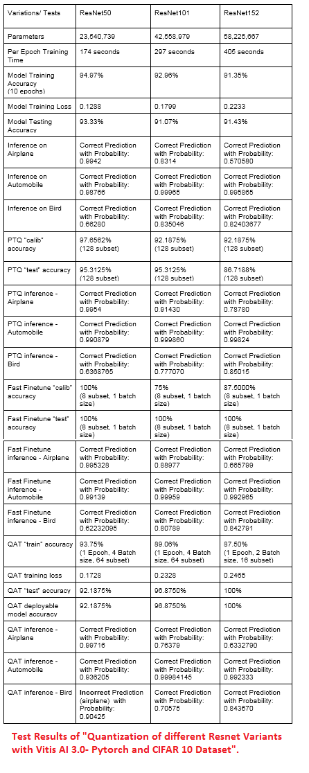
Test Results is in attachment!

Compilation of Resnet Variants:

Compilation is straight forward, we just need arch.json (or DPU architecture) file and then we can run Vitis AI compiler (VAI_C) for Quantizing model. All the modification, tweak and changes needed on Quantization. Arch.json can be obtained from the MPSoC Board terminal by running (show_dpu and xdputil query), if you are using ZCU102/ZCU104 or KV260 Boards then you can follow this Board Setup link [https://xilinx.github.io/Vitis-AI/3.0/html/docs/quickstart/mpsoc.html] and get arch.json respectively.

For compilation this script can be followed [reference link]:

  vai_c_xir \
  --xmodel      <Quantized_Model_Directory>/quantized.xmodel \
  --arch        <arch_json_directory>/arch.json\
  --net_name    CNN_<net_name> \
  --output_dir  <directory>/compiled_model

Reference of this tutorial are: UG1414-AMD-Xilinx and Vitis AI (3.0) Github.

For complete sources and test results, check LogicTronix/Vitis-AI-Reference-Tutorials/tree/main/Quantizing-Resnet-Variants

Kudos to our Team, Jinu Nyachhyon for this tutorial!