AI at the edge involves loading machine learning models onto microcontrollers that enables them to make far "smarter" decisions on a broader range of data than a traditionally programmed device. This project is about how to get started with this technique using one of QuickLogic's QuickFeather Development Kits and the suite of SensiML tools for gathering data, creating a model, and deploying it. It's a really useful tool for the likes of scientists, engineers, and hobbyists to tackle large issues such as climate change. If that interests you, take a look at the current Challenge Climate Change contest, where everyone is encouraged to use the QuickFeather with SensiML to solve problems like reducing energy consumption or early wildfire warnings.
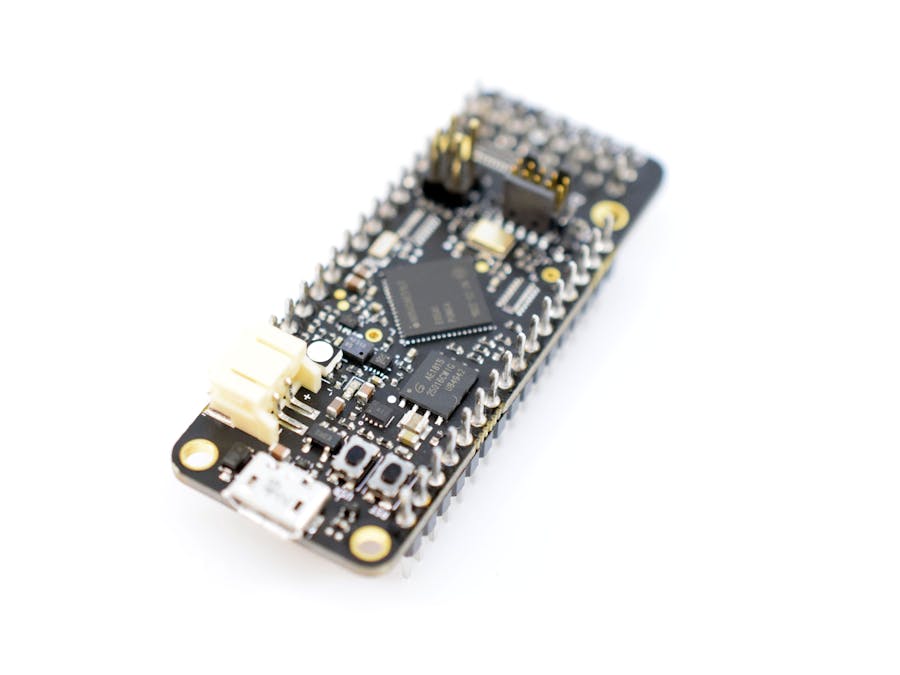
The QuickFeatherThe QuickFeather Development Kit is an impressive device that packs tons of functionality into a small footprint. Here are some of the specs:
- QuickLogic EOS S3 processor (the first FPGA-enabled Arm Cortex-M4F MCU to be filly supported with Zephyr OS)
Externally connected:
- 16Mb of flash memory
- mCube MC3635 accelerometer
- Infineon DPS310 pressure sensor
- Infineon IM69D130 PDM digital microphone
All with the footprint and layout of the standard Feather specification.
Before you begin with anything else, you'll need to get your QuickFeather the latest binary, which takes just a couple of steps to do. First, download the latest .bin file from here, and make sure to select the one for Simple Stream collection, not the MQTT-SN one. Then use git clone to download the TinyFPGA Programmer Application with git clone --recursive https://github.com/QuickLogic-Corp/TinyFPGA-Programmer-Application.git and then pip3 install tinyfpgab which installs the Python library. It requires a Python version at or above 3.6, so keep that in mind.
After placing that .bin file from earlier into the folder you just saved the clone into (it should contain tinyfpga-programmer-gui.py), plug in the device via USB and press the 'Reset' button on the QuickFeather, then the 'User' button within five seconds after that. This causes the LED to begin flashing green, and indicates the board is in upload mode. Run the command python tinyfpga-programmer-gui.py --port COMX --m4 quickfeather-simple-stream-data-collection.bin --mode m4 to flash the binary file over USB, where COMX is the COM port for the QuickFeather. After the program has finished uploading, press the 'Reset' button to load the new application. The LED should blink blue for five seconds and then turn off once it's done.
SensiML Data Capture Lab (DCL) is what lets data be captured from the device and transported to the host computer, where it can then be processed further and exported. To begin, create a new account and download the DCL software, as well as sign in.
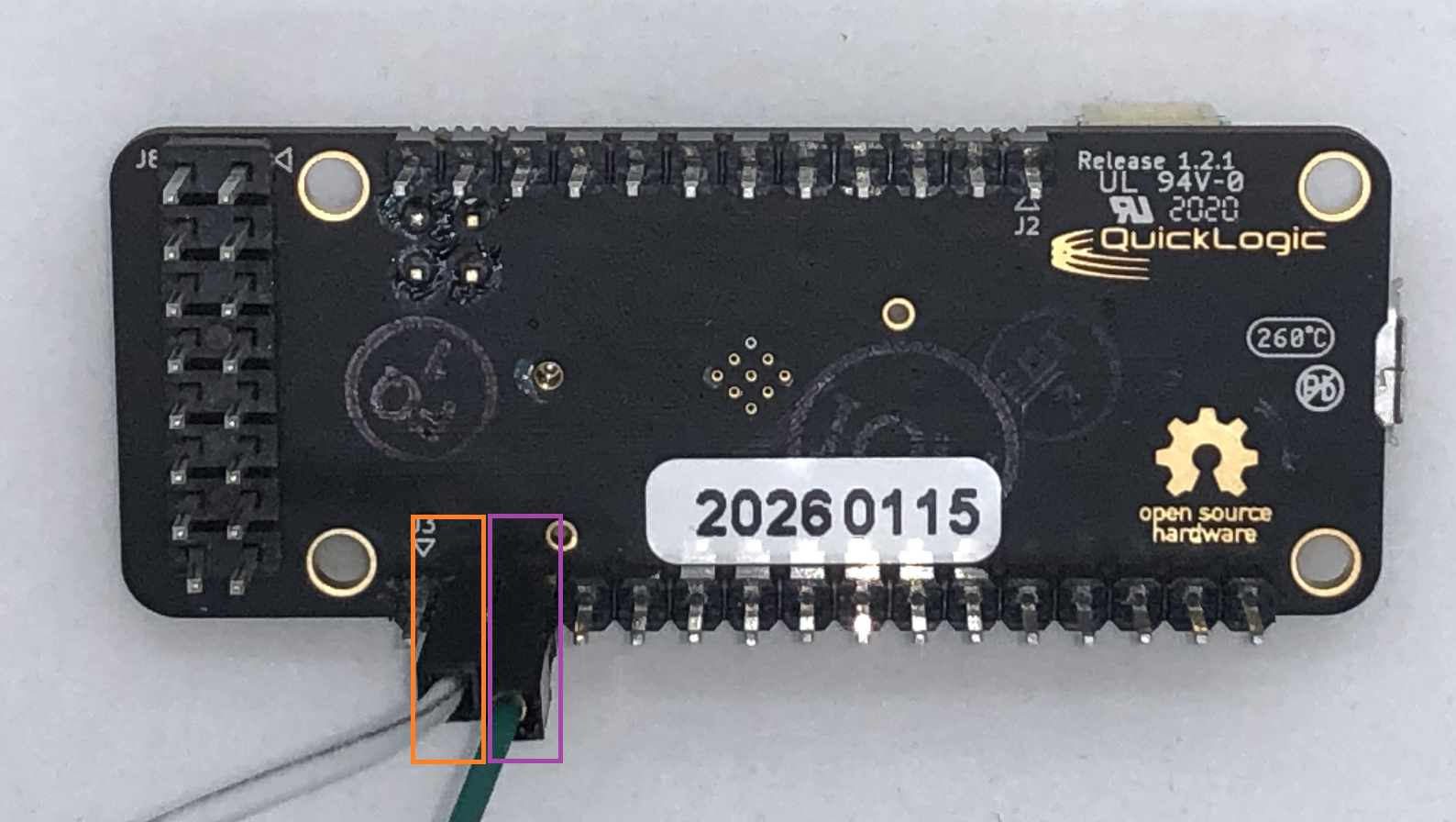
Simple Streaming capture mode requires the use of the UART pins on the QuickFeather, so connect a USB to TTL serial adapter like so:
where the pin highlighted in orange is the adapter's RXD pin, and the one in purple is the adapter's TXD pin. It communicates over a baudrate of 460800.
Within the DCL, create a new project by giving it a name and saving it somewhere.
Then switch from the 'Label Explorer' mode to 'Capture' mode. The DCL uses plugins in the form of SSF files that tell it how to communicate with devices. Download the one for the QuickFeather here (make sure to choose the one for Simple Streaming) and add it using Edit->Import Device Plugin and selecting the just-downloaded SSF file. In the upper-right corner you'll see the Sensor Configuration is empty, so click on the add new sensor button, select the QuickFeather Simple Stream plugin, use the 'Motion' capture source, a sample rate of 105 samples per second, and ensure that 'Accelerometer' is checked. Go ahead and save it as 'Sensor 1'.
The Data Capture Lab comes with some nice features that allows it to be extremely versatile. Probably the most important one is the ability to capture data from almost any board with any sensor attached, rather than having to wait for it to become officially supported. This can be accomplished by creating a custom SSF file that specifies the capabilities and configuration of that board. You also have the option to add metadata to your captures, which can function as labels, such as splitting training data based on more specific parameters or telling training and testing datasets apart. Finally, the data that's been collected can be viewed in a large number of different ways, such as splitting axes apart onto separate graphs, or splicing captures together. There are many more features as well, so to read more about them, visit this page.
A Sample ProjectBecause this project is just for getting started, we won't get to some of the more advanced features in the software, but we will go over the most pertinent ones. The resulting dataset will be small, and that's fine for this project because we're only interested in determining whether there is movement or the board is at rest.
Capturing DataWith the board set up, go ahead and click "Connect" within the DCL after finding the correct serial port (the one for the USB to TTL serial converter!) with the "Scan Devices" button. If it doesn't work initially, try unplugging the converter and plugging it back in, or disconnecting and reconnecting.
Just below that pane there is a section for adding labels and metadata. I added my two labels: rest and movement. Then for the metadata I added a Class and chose two values: Train and Test, which denotes each capture as either for training or for testing.
After capturing my data by pressing the Record button at the bottom, I needed to clean it up a bit and ensure that only data that represents the feature(s) I'm trying to isolate makes it in, i.e. no "resting" within the movement data.
This can be accomplished by going to the Project Explorer tab in the upper-left and double-clicking on the capture you want to modify. Then you can add segments by dragging your mouse while holding down right-click over the areas you want to keep. The more times you do this, the more segments will be added.
You can see them in the upper-right area. This also allows you to capture different labels within the same capture by creating segments for each of them and changing the labels.
After heading to File->Close FIle, it's time to use the Analytics Studio to generate a model from the captured data. Remember that data saved within the DCL is automatically uploaded and stored in the cloud, although it might take a few moments for it to refresh and appear.
Training a ModelWe begin by going to the Analytics Studio in a web browser and selecting the project that was created in the DCL.
To train a model, we must first tell the Analytics Studio which data we want to use in the form of a Query. This can be done by clicking on the Prepare Data tab and entering a name, session, label, relevant metadata, the sensor(s), and how to plot it. After saving the dataset should appear on the right, and we can see how many segments are in each label.
Pipelines can be constructed by going to the Build Model tab and entering a name, the query that was just created, window size (make it the same size as the capture rate for the sensor), optimization metric (f1-score is the most balanced), and the classifier size, which limits how large the model can be, great for loading onto ROM-constrained chips. Clicking Optimize will go through and build the model, and depending on how large the dataset is, it might take a while to complete.
The final step in this process is deployment, which comes in the form of Knowledge Packs. Think of them as containers that hold your model and the associated data about it. They come in three flavors: binary (pre-built, just flash to the board and run), library (easily add it to your project and interface with an API), or source code. For this project, we'll just be building a binary, so in the Download Model tab select the pipeline you just optimized, along with the following target device settings:
- HW Platform: QuickFeather 1.5.0
- Target OS: FreeRTOS
- Format: Binary
- Data Source: Sensor 1 (the onboard accelerometer)
- Output: Simple Streaming (via UART pins)
Pay attention to the class map as well. In this project, a result of 1 means movement, and a result of 2 means rest. Download the zip file and extract the binary file to the same folder that contains the Python file used earlier for flashing the Simple Stream firmware. With the QuickFeather back in upload mode, run the same command from before, except this time replace quickfeather-simple-stream-data-collection.bin with the name of the knowledge pack binary. Opening up a serial monitor with 460800 baudrate will show the classification output of the model, and as seen below, it works!
If using machine learning at the edge interests you, then check out the Challenge Climate Change contest and request a free QuickFeather board. Then go have a look at some documentation and see what sensors and or components you can add to help solve one of the most important problems currently facing us.


Comments
Please log in or sign up to comment.