Wells: A UV-C Disinfection Robot for Indoor Spaces

Overview

The 2019 Novel Coronavirus (COVID-19) rapidly spread across the globe, plunging many countries into lockdowns in order to prevent further spread and an overflow of the healthcare system. As the world reopens, there is going to be a growing demand for projects that utilize cutting-edge technology in order to further aid in public health and safety efforts.

Wells, named after sanitary engineer William F. Wells, who was the first to apply UV-C light to disinfect environments, is a low-cost robot designed to autonomously sanitize environments using UV-C Radiation. Wells measures in at 16" x 20" x 26" (L x W x H) for high maneuverability, weighs ~40 lbs, and uses mecanum drive wheels for agile omnidirectional motion. It uses 2 high-power 36W UV sanitization bulbs to sanitize regions of up to 4 meters in diameter, and is able to sanitize regions to the specified kill dose within 120 seconds (Appendix A). The robot is outfitted with a RPLIDAR sensor, which it uses for Simultaneous Localization and Mapping (SLAM) when exploring a new environment, and for Particle Filter-based localization when sterilizing a mapped environment. In addition, it features various safety features, including the ability to use the LIDAR to instantly shut down the bulbs when motion is detected, and the use of bump switches on all four sides of the robot to shut down if the robot touches anything. The robot features a 12v 10 Ah battery, with an approximate battery life of 30 minutes. The battery is hot-swappable, and can be charged in under 1 hour.

All of this project is available under the CERN-OHL-P V2 license (available at https://ohwr.org/cern_ohl_p_v2.txt)., and all files and documents (including BOM with descriptions and visualizer source folder) can be found here.

Design Requirements & Constraints

The robot's main design constraints were:

• It had to be durable
• Custom parts had to be easily sanitized
• It had to be accessible
• It had to be capable of fully autonomous motion, and shut down when motion is detected
• It had to scale to mass production

In order to meet these constraints, we used high-quality 6061 aluminum parts, maximizing use of off-the-shelf components when possible, and when we had to use custom components we used ones that could be sourced from sendcutsend.com cheaply or other suppliers. We also equipped the robot with an array of sensors, in order to efficiently localize the robot and detect movement.

We chose the parallel-plate design primarily for sanitation and accessibility reasons -- robots designed with additive manufacturing (i.e. 3d printing) can have bacteria and contaminants get trapped between layer lines during the printing process, which poses a health and safety risk. Within subtractive manufacturing (machining, waterjet, etc.), we tried to have parts that could be manufactured with online services in a cost-effective manner, and hand tools, such that it would be accessible to people who don’t have direct CNC access, and as such went with a plate construction over billet or extrusion construction, which are extremely expensive.

In addition, metal plate parts are the easiest to mass-produce, as 3d printing and CNC milling are expensive and time-consuming at scale.

Robot Design

The robot consists of two major components -- the chassis and the superstructure. The chassis, which drives the motion of the robot, consists of four 4" diameter mecanum wheels, each driven by an AndyMark Neverest 40 Gearmotor with a 5.44:1 gear reduction. The mecanum wheels provide a force vector at 45 degrees to the axis of rotation (Figure 1), and by moving in different directions enable the robot to move in any direction, irrespective of its orientation. This greatly simplifies controls, and enables smooth motion from point to point.

The chassis uses a parallel-plate 6061 aluminum construction, with COTS (Commercial Off-The Shelf) Standoffs and brackets used to connect the plates. This ensures that the chassis is structurally sound, reducing the likelihood of failure and the need for constant maintenance.

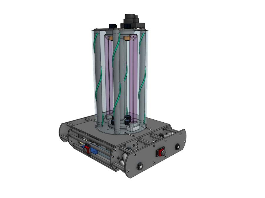
The superstructure is mounted directly on top of the chassis using COTS brackets, and consists of the UV Bulbs, as well as the RPLIDAR sensor that enables the robot to localize itself relative to its environment, and NeoPixel indicator RGB LED strips. Structurally, the 6061 aluminum plates are held together with four large standoffs made with round tube and tube insert nuts, as well as a fifth tube running down the center attached with COTS mounting brackets. The UV bulbs are supported by an aluminum plate mounted to the center column, and are protected from outside impact with a wire mesh cage (modeled here as a transparent ring).

Software Stack

This project is built around the ROS framework, which is an open-source project that uses a modular system to enable development of scalable robotics software. As the ROS website states:

The Robot Operating System (ROS) is a flexible framework for writing robot software. It is a collection of tools, libraries, and conventions that aim to simplify the task of creating complex and robust robot behavior across a wide variety of robotic platforms.

By using the ROS framework, this project is able to use advanced visualization tools, cutting-edge localization packages, and more, all within one standard ecosystem. In addition, this adaptive framework allows for the robot to simultaneously log data (i.e. bulb voltage), and visualize the path a robot takes on a sterilization run real-time, for effective diagnostics.

The ROS topic infrastructure enables management and communication of multiple programs running simultaneously. This is key to safety, as it enables rapid response to environmental changes which allows the robot to shut off the bulb virtually instantly when motion is detected.

Navigation&Control

This project uses a custom-written path generation & visualization tool (Appendix B), and then follows the paths autonomously using a PID controller (Appendix C). This approach was taken over a coverage path planning approach due to the "stop and go" nature of movement in this situation, which traditional coverage planning algorithms don't consider.

To start, maps of the environment are first generated using using the GMapping SLAM package, with the robot being driven around the area to be mapped. Once the map is generated, it can be used with the path visualizer tool in order to generate a series of waypoints (or points where the robot stops and exposes the region to UV light) for the robot to follow. From there, the list of waypoints can be loaded onto the robot, and the robot will autonomously follow the path with a PID controller, stopping at each waypoint for two minutes to irradiate the selected area. The robot uses the AMCL probabilistic localization package during operation, which implements an adaptive Monte Carlo localization approach with a Particle Filter to localize the robot relative to the environment. While it is moving, the robot will log data on bulb life, robot path, and more.

Safety features

This robot is equipped with a range of sensors and other devices to ensure operational safety. When on, the robot uses its buzzer and LEDs to indicate operational state (either emergency stopped, disabled, enabled without UV or enabled with UV On). In addition, it uses the RPLIDAR sensor to check its surroundings and will automatically enter an "emergency stopped" if motion is detected by the RPLIDAR or if one of the four bump sensors is triggered.

When this state is activated, the robot will send a message to the console, and won't re-start until an operator manually clears it. This functionality exists in order to ensure that it does not accidentally re-start itself with a human or animal in the vicinity.

Appendix

AppendixA:UVDoseCalculations

While irradiance is normally an empirically measured quantity, this project required an estimation to ensure that the hardware was capable of quickly sanitizing a given area. To estimate the irradiance, the point source model was used. Irradiance can be estimated by dividing the total UV output power by the area of exposure. The UV output power was estimated to be 27W (assuming 75% bulb efficiency), and the exposed region was assumed to be a circle with a radius of 2 meters and an area of approximately 12.57 square meters.

Based on this, the irradiance was calculated to be 2.148 W/m^2, or approximately 214.8 µW/cm^2. Therefore, the dose at 2 meters for an exposure time of 120 seconds would be 25.8 mJ/cm^2. This satisfies the requirements, as based on this technical report (Kowalski, Walsh, & Petraitis), the average D90 dose for 90% inactivation of coronaviruses is 237 J/m^2, or 23.7 mJ/cm^2.

In addition, this robot is capable of taking on even the most resistant viruses should another outbreak occur, since the highest D90 dose for inactivation in the report (for SARS coronavirus Urbani), is 2410 J/m^2, or 241.0 mJ/cm^2, which this is able to match at just under 19 minutes of exposure.

Since the robot is capable of shutting down within one second (with an exposure of 0.21 mJ/cm^2) due to the ROS framework, it will never exceed the threshold limit value of 3.1 mJ/cm^2 before shutting off the UV bulb completely. (source: http://web.mit.edu/cohengroup/safety/uv110720safety.pdf).

AppendixB:PathVisualizer

For this project, a custom path visualizer was written as a proof of concept. All of the visualizer files can be found in the folder linked in the introduction. This path visualizer is designed for systems running Ubuntu 18.04, with ROS Melodic and the map_server package installed. To run the path visualizer:

0. Open the Terminal. This can be done with the shortcut:

ctrl+alt+t

Or done from the "Activities" menu.

1. Start ROS. This can be done with the command:

$ roscore

2. Navigate to the directory the visualizer and map files are in, and Initialize the map_server. To run the map server, you will need a map generated with GMapping(in the form of a.pgm and.yaml file). For testing, the real-floor0 map was used, from the University of Washington's MuSHR simulation project.

$ rosrun map_server map_server real-floor0.yaml

3. Start a static tf transform publisher. This initializes the coordinate frame that provides a frame of reference for the visualizer's coordinate system

$ rosrun tf static_transform_publisher 0 0 0 0 0 0 1 map world 100

4. Make visualizer.py executable. This is so that you can run the program directly from command line

$ chmod +x visualizer.py

5. Launch visualizer.py

$ ./visualizer.py

6. Launch RViz. This is the GUI environment that will let you see the visualized path

$ rviz

7. Once inside RViz, your window should look something like this :

Now that RViz is open, navigate to the "Add" button in the bottom left corner. Click on it, and in the menu that opens, click on the "By topic" tab in the top right. Select MarkerArray under /visualization_marker_array, and click "OK".

8. To add points to your path, simply click "Publish Point" in the top menu, and then click on the map wherever you wish to add your first waypoint. This should create a circle, representing the irradiated region, as well as a smaller square, representing the area covered by the base of the robot.

9. To add more points to your path, repeat the steps outlined in step 8. As you do so, you should also see arrows drawn between each circle, visualizing the movement of the robot.

10. When you are done, simply close the visualizer, and all of the points will be saved to a text file called path.txt, which can be loaded onto the robot.

AppendixC:PIDController:

For an introduction to PID control, please refer to Chapter Two of this book.

The main difference between a basic PID controller for a linear system and the controller used for this type of holonomic position control is that the error function becomes a vector-valued function, with the error being defined as the vector starting at the robot's current pose and ending at the robot's target pose. From there, a target velocity vector is generated using the PID equation, where u(t) is the desired velocity vector at time t, and e(t) is the error vector at time t

Finally, once a desired velocity vector has been generated, the robot uses the kinematic model defined in section 12.4.2 of the linked book to generate individual wheel velocities

Appendix D: Manufacturing&Electronics

All parts can be assembled using hand tools (hacksaw, riveter, allen keys). Exploded view drawings can be found in the folder with the BOM files. All electronics, as well as the front/back push-button sensors, are held down using zip-ties or VHB Tape. Electronics are labeled in the CAD, since block models were often needed to represent them, and descriptions can be found in the BOM. The LED strips need to be cut according to the guidelines on their website, and wrapped around the support pillars like in the CAD