Magnetically Levitated Ball with MATLAB and Arduino

Description

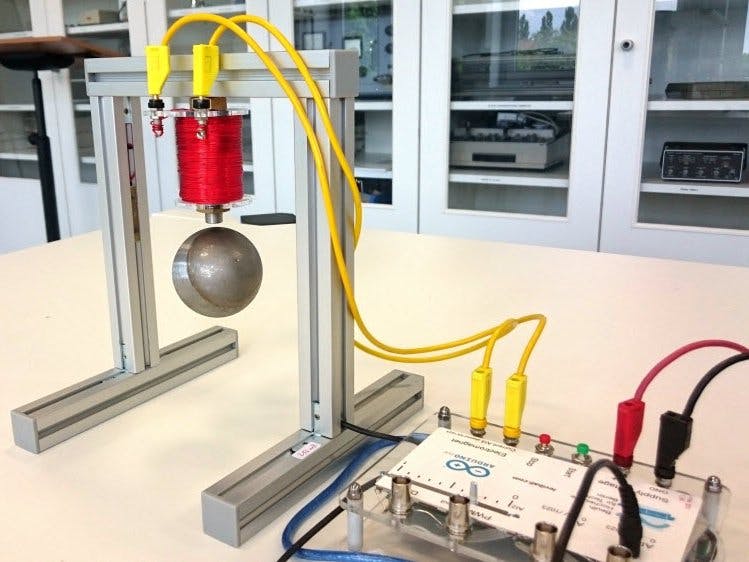
A magnetically levitated control system (Maglev) is realized in a well-known way: an iron ball is held in levitation with the magnetic force of an electromagnet. This experiment has been built up numerous times before and is widely available on the internet. Our focus however was to set up a real time control loop which is only programmed in Simulink. Therefore, we are using the Arduino Due Board.

A constant loop time is essential for digital feedback control. Normally a micro-controller is programmed using interrupt routines. We applied the Simulink Support Package for the Arduino Hardware and achieved a feedback control system with a constant control loop frequency of up to 1 kHz. We could implement and test different control algorithms on real Maglev systems without writing any C-code.

Prerequisites

• MATLAB Simulink (2013a or newer)

• Simulink Support Package for Arduino Due Hardware (we used version 14.1.3)

Downloadable Code and Models

https://mathworks.com/matlabcentral/fileexchange/61131-pid-control-with-simulink-and-arduino

Required Hardware

• Magnetic coil (core diameter 14 mm, length 60mm, 1700 windings 0.6mm wire), but many other coils will also work

• Ball (ferromagnetic material (iron or steel), diameter 60 mm, mass 200 g, we ordered them from ball-tech.com)

• Sensor (IR-Diode VSMB 2000X01, Photo diode BPW34FS (5x))

• Power electronics (FET FDB580, Diode (50V, 2A))

• two rail2rail OP (e.g. AD8646) and some passive electronics

• Arduino Due

Tasks

The principle of the magnetically levitated ball is shown here.

The gap between the electromagnet and the ball is measured using a light sensor. The Arduino board acts as a PID-controller and calculates the voltage, which is necessary to force the ball magnetically into the levitating position.

Task 1 Mechanical system: We used Al-profiles (25x25mm) to build the frame. All non-ferromagnetic materials will work but the coil must be fixed (no elastic movement is allowed).

Task 2Sensor: The gap between the coil and the ball is measured with infrared light. To receive the light from the IR-LED (on the opposite side) we used five photodiodes arranged in a line as shown below.

We got nearly linear values for gaps between 1 and 9 mm. The circuit for the sensor electronics is fairly simple, as shown in the figure.

You will find many alternative solutions on the internet. The left OP transfers the light current into a voltage, the right OP is used to adapt the gain. Both OPs must be rail2rail! Be careful with the output voltage; do not exceed 3.3V to protect the Arduino input from damage.

These electronics have the disadvantage, that all ambient light will influences the measured value.

So we found a better solution with modulated light shown in the schematics below.

The oscillator gives AC-current with a frequency of 100 kHz to the LED. The light receiver amplifies only the information which has passed the band filter. Therefore, the surrounding (DC-) light does not influence the measured signal.Of course this circuit is more complicated to replicate, but it works much better than the upper one. The schematic can be found on leviball.com.

Task 3Arduino Board: Only a few connections are needed: power supply (+5V and GND), analog input (AI4) and PWM output (PWM 9). The 3.3V-Pin of the Arduino board can be used as the power supply for the sensor circuit.

We have connected another analog input pin: a variable input voltage was generated with a potentiometer to adjust some parameters of the controller (see below for the schematic diagram).

Task 4Power Transistor: The PWM-output of the Arduino board directly drives the gate of the power transistor. All red wires should be short and not too thin, because sharp current impulses must be handled. During the off-state of the transistor the current of the coil flows through the diode. Don’t forget the diode!

For our setup we applied the integrated full bridge DRV8801PW. So we can use the integrated thermal protection. Also we are able to measure the current to use this for state space control.

Task 5Feedback control: A control loop must run with constant clock rate. It must be much faster than the (inverse) time constants of the controlled system. We were looking for a very easy way to program the Arduino board, therefore looking for a way to avoid developing programming code with interrupt routines and complicated timer structures.

So we used Simulink in combination with Support Package for Arduino Hardware. A very simple Simulink model will fulfill all our needs.

It can be downloaded directly from Simulink to the Arduino Due board and will run alone also after disconnecting the USB-cable. The structure is very similar to a usual control loop.

• The sample rate of the loop is determined by the source blocks as they are the Step and the Analog Input. The lowest value was a sample time of TS = 0.001, that means 1 millisecond, we were able to test without failure in loop processing (on Arduino Due, other Arduino boards may be not so fast).

• Choose for the Step block: Step time = 0, Initial value = 0, Final value = set point of your levitating ball, (we worked with 0.006 (distance in meters)), Sample time TS = 0.001 is the same as before

• For the analog input block choose the correct input pin number (we used 4) and the same sample time.

• The Gain blocks in the plant-rectangle must be adjusted to your plant. The PWM-signal will accept values between 0 and 255, that’s why we have added a saturation block. The Offset of 127 is only necessary for our variant with a full bridge. With only one switching transistor you don’t need the offset.

• The analog input blocks value is 1023 at 3.3V input level.

• To realize the PID controller we used the mathematical term below — this can be found in the Simulink structure. Only three parameters need to be defined: proportional gain KP and two time constants TI (integrator) and TD (differentiator). For your setup you must test suitable values, we got good results with TD=0.05, TI=0.5 and KP = -3000.

• Downloading the model to the Arduino board needs some time. To find the right PID-parameters several downloads will be necessary. We developed a good way to adjust our parameter during testing: As already mentioned we used a potentiometer, which is connected to an additional analog input port.

So we got a variable value between 0 and 1023. We divided it by 512 (this gives values between 0 and 2) and multiplied – for instances – the gain factor KP with this value. So it will be very easy to find good parameters for the PID controller.

Summary

The described Simulink model can be applied for many tasks with feedback control. We use it especially for educational purposes: Our students are familiar with modelling in Simulink. This way they can confirm their results in practical setups and focus their minds on subjects of control engineering without developing any program code, interrupt routines or hardware registers.

The presented Simulink model can be extended very easily. We have also successfully tested complex control structures like state space controller, controller with state observer and a nonlinear control algorithm.