Using YDLIDAR with TI TMS320F28379D

This is a portion of my final project of SE423 at UIUC. The full project can be found at https://www.hackster.io/yixiaol2/robot-car-path-planning-with-motion-tracking-and-lidar-5d5ba3. For this final project, I write code for the F28379D launchpad to process the raw Lidar data with the help of professor Dan Block.

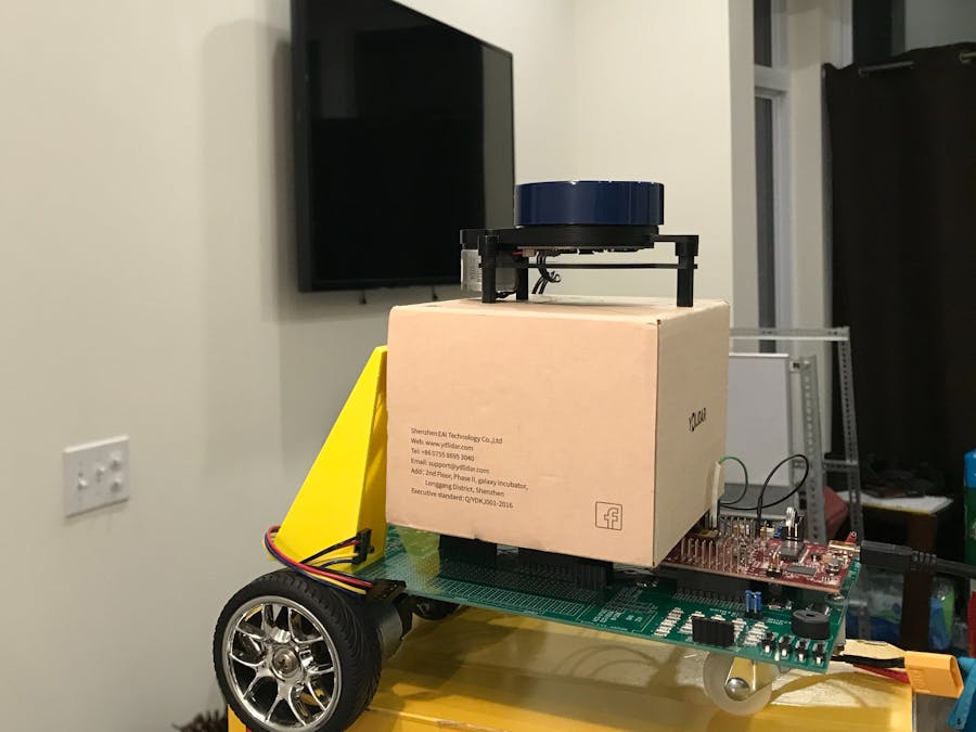
Understanding YDLidar X2

YDLidar X2 is a cheap Lidar that performs well enough for the purpose of my project. It can sense a range of 0.10 to 8.0m, with a 360° perspective. Another great thing about this Lidar is that it will automatically start to collect data the instant it is powered on.

I played around with the simple software provided on their website in the living room of my apartment. The data from the software is in the form of Angle, Range, and Intensity, below is a figure of the data from the provided software. Angle and Range correspond to the angle and distance of the obstacle that reflects the laser beam. In this project, we only need Angle and Range.

With that data, it is easy to reproduce the plot from the software with Matlab. Below is a plot of my apartment's living room and a setup for collecting the data.

However, for our project, we need to process the raw data spitting from the Lidar with the F28379D launchpad instead of interfacing with the provided software. It took me some work to get this part done. Based on the development manual, the data is sent in hexadecimal to the serial port of an external device according to the below data structure.

The data from the Lidar is transmitted in packets. Each packet contains a header(always 0x55AA, 2bytes), a type(1byte), a number of samples (1 byte), a starting angle(2 bytes), an ending angle(2 bytes), a check code(2 bytes), and sample data (2 bytes each), indicating the distance. The total number of sample is usually 40, so there will usually be a total of 2+1+1+2+2+2+2*sample number(usually 40) = 90 bytes of data a packet. The starting and ending angles indicate the angles of the sample data. After partitioning the angles, we can get the correspondence of the angle and the distance data.

Read the Lidar data

After understanding the data structure, we can connect the Lidar with our launchpad. Since the data is transmitted through the serial port, we chose pin 9 of the launchpad, which corresponds to SCID, to receive data from the Lidar.

I chose to use a large state machine to keep track of the data coming from the Lidar. Since all the data coming from the serial port is in char (1 byte), I created the state machine based on each byte received.

Since all the packets start with 0x55AA, with the LSB (0xAA) coming first, then the MSB (0x55), I created the first two states only to recognize the header of the packet. It will keep reading when seeing the correct header, otherwise, it will exit and keep waiting for the header.

if(state == 0) { //check 0xaa
        if(data == 0xAA) {
            state = 1;
        } else {
            state = 0;
        }
} else if (state == 1) {//check 0x55
        if(data == 0x55) {
            state = 2;
        } else {
            state = 0;
        }
}

After getting the header, I used 1 state to detect the packet type (should be 0x0 in our case, as it is point cloud mode), 1 state to get the sample size.

else if (state == 2) {//check 0x0
        if (data == 0x0) {
            state = 3;
        } else {
            state = 0;
        }
} else if (state == 3){ //read sample size
        sampleSize = data;
        state = 4;
}

It is a little complicated to read the angle data, since the angle data contains 2 bytes, while we can only read one at a time. Also, there's a conversion formula for the raw angle given in the development manual:

To get the angle, I first read and store the LSB, then combine it with the next byte, which is the MSB of the angle, then combine them to get a 2 bytes angle value. Then based on the formula, the actual angle is given by the angle value right-shifted 1 bit and divided by 64. Notice that the angle value needed to be masked with 0x7fff, since it is only 15 bits after a right shift of 1. Also, the angle value is a float number, so divided by 64.0 is necessary. Normally, the angle difference is around 30 degrees, but there are cases that the starting angle + 30° > 360°, then the ending angle will starts from zero, which will cause some problem for later partition of the angle, so I added 360 to the ending angle when the ending angle is smaller than the starting angle.

else if (state == 5) {//record starting angle
        start_angle = ((((data<<8)| startangleLSB)>>1)&0x7FFF)/64.0; //get the starting angle
        state = 6;
} else if (state == 6) { //read end angle
        endLSB = data;
        state = 7;
} else if (state == 7) {//record end angle
        end_angle = ((((data<<8)| endLSB)>>1)&0x7FFF)/64.0;  //get the ending angle
        //make sure the end angle is greater than the staring angle
        if (end_angle < start_angle) {
            cor_end = end_angle + 360;
        } else {
            cor_end = end_angle;
        }
        //calculate the difference between the start and end angle
        delta_angle = cor_end-start_angle;
        state = 8;
}

Then there's only check code and actual sample data left. Here, I ignore the check code for simplicity, so after entering state 8, we waited for 2 more bytes to come, then started to collect the sample data, which corresponds to the distance. For distance, it is also 2 bytes, so similar to the angles reading, I created a smaller state machine inside state 8 to first store the LSB, then combine it with the MSB value of the sample data reading. From the development manual, the distance is the sample data/4, in mm. When the number of sample data is equal to the number of samplesize we got from state 3, we are done with the current packet, and can go back to state 0 to wait for the packet header. The below code also contains data storage, which will be discussed in the next section.

else if (state == 8) {//record samples and ignore the check code
        //postion is 0 when entering
        if(position > 1) {
            if (dis_state == 0){
                dLSB = data;
                dis_state = 1;
            } else if (dis_state == 1){
                float dist = (((uint16_t)data<<8 | dLSB))/4.0; //calculate the distance
                pts[arrayIndex].distance = dist;
                pts[arrayIndex].timestamp = numTimer0calls;

                //calculate the raw angle
                float raw_angle = (delta_angle)/(sampleSize - 1) * (sampleindex) +start_angle;
                sampleindex = sampleindex+1;
                if(sampleindex == sampleSize) {
                    sampleindex = 0;
                }
                pts[arrayIndex].rawAngle = raw_angle;
                //calculate the calibrated angle
                if(dist == 0){
                    cal_angle = raw_angle;
                } else {
                    cal_angle = raw_angle + atan(21.8*(155.3-dist)/(155.3*dist))*57.296-90;
                }
                pts[arrayIndex].cor_angle = cal_angle; //need to consider the 0 degree of the lidar is not the same as the x direction of the robot car
                //not sure it will work as expected yet

                //use a pingpong buffer to keep the data
                if (pingpongflag == 1) {
                    pingpts[360-((int16_t)(cal_angle + 360.5))%360].distance = dist*FEETINONEMETER*0.001; //in feet
                    pingpts[360-((int16_t)(cal_angle + 360.5))%360].timestamp = numTimer0calls;
                } else {
                    pongpts[360-((int16_t)(cal_angle + 360.5))%360].distance = dist*FEETINONEMETER*0.001; // in feet
                    pongpts[360-((int16_t)(cal_angle + 360.5))%360].timestamp = numTimer0calls;
//                    if (write_matlab_data == 1) {
                        matlab_dist[360-((int16_t)(cal_angle + 360.5))%360] = dist*FEETINONEMETER*0.001;
                        matlab_count += 1;


//                    }
                }
                dis_count += 1;
                dis_state = 0;
                if (arrayIndex < 599) {
                    arrayIndex += 1;
                }
            }
        }
        position += 1;
        //when done all the readings
        if(position >= sampleSize*2+2) { //the total number of bytes for check code(2) and sample data

            if (checkfullrevolution == 0) {
                checkfullrevolution = 1;
                anglesum = delta_angle;
            } else {
                anglesum += delta_angle;
                if (anglesum > 360) { //when it goes more than a 360 degrees
                    checkfullrevolution = 0;
                    if (pingpongflag == 1){
                        UseLIDARping = 1;
                        pingpongflag = 0;
                    } else {
                        UseLIDARpong = 1;
                        pingpongflag = 1;
                        if(matlab_count >= 360) {
                            write_matlab_data = 0;
                        }
                    }
                }
            }
            position = 0;
            state = 0;//enter state 0 to read new packet
            GpioDataRegs.GPATOGGLE.bit.GPIO9 = 1;
        }
    }

Store the interpreted data

Since we want to know the angle and the distance of the points that we detected, I created a structure called data_pt to store the distance, timestamp, and angle of the data point. distance is the number we calculated from state 8; timestamp is the number of times CPUTimer0 is called; while for angle, we need to use the angle correction formula, since it takes longer for the laser from a more distant object to travel back. Therefore, the angle in the structure data_pt is actually two variables, the raw angle, and the corrected angle. For the raw angle, we need to use the intermediate angle solution formula.

And for the corrected angle, we need the below formula.

To store the data, I created a 600 data_pt buffer array, then passed all the calculated values from state 8 into the data_pt array. This buffer array is not ideal for later processing since the data is organized in the order of receiving instead of the angle or distance. Therefore, I created another structure dis_time to only store the distance and timestamp. Then, a ping-pong buffer is used to make sure the processor has enough time to process and store all the data. They both have 360 dis_time entries, and the index of the ping-pong buffer corresponds to the angle of the sample points. That is, pingpts[x] will contain the distance of x degree and the timestamp when of the x degree's reading. Therefore, we only need to cast the corrected angle to the corresponding index, and we can store the distance and timestamp in the pingpts and pongpts array. There are around 400 points for each lidar rotation, keeping 360 of them is good enough for our project purpose, so we simply truncated the angle data.

//use a pingpong buffer to keep the data
if (pingpongflag == 1) {
    pingpts[360-((int16_t)(cal_angle + 360.5))%360].distance = dist*FEETINONEMETER*0.001; //in feet
    pingpts[360-((int16_t)(cal_angle + 360.5))%360].timestamp = numTimer0calls;
} else {
    pongpts[360-((int16_t)(cal_angle + 360.5))%360].distance = dist*FEETINONEMETER*0.001; // in feet
    pongpts[360-((int16_t)(cal_angle + 360.5))%360].timestamp = numTimer0calls;
    matlab_dist[360-((int16_t)(cal_angle + 360.5))%360] = dist*FEETINONEMETER*0.001;
    matlab_count += 1;
}

Finally, we got the Lidar readings storing in the ping-pong buffer array, with the index of the array equals the angle of the points counting from the 0 degree of the Lidar, and the content includes the distance of the points at that angle, which is the same as the output from YDLidar's original software. To visualize this data, we can plot it by storing the memory using CSS, and pass those values in Matlab. Here, I got code from Professor Dan Block to store the values in Matlab array.

The below figure is the result of plotting the points when placing the robot car in a built track in our lab. For my complete project, I did coordinate transformations to make a"global view" of the track, given the location and angle between the robot car and the "x-axis" (which is the horizontal line in the figure). This figure is generated with the robot car having an angle of 30° with the "x-axis". As shown in the right figure.

The initial condition is set at the beginning of the file.

//initial condition
double pose_x = -4; //x_position of the robot car
double pose_y = 6; //x_position of the robot car
//need to put negative initial angle because the Lidar is rotating CW
double pose_theta = -30; //angle of robot car
double pose_rad; //angle in rad

Credits

Thanks to Professor Dan Block for helping me debug and figure out how to interpret the data.

Thanks to Scott Manhart for designing the Lidar stand.