Estimating Pi with the Monte Carlo Method

Introduction

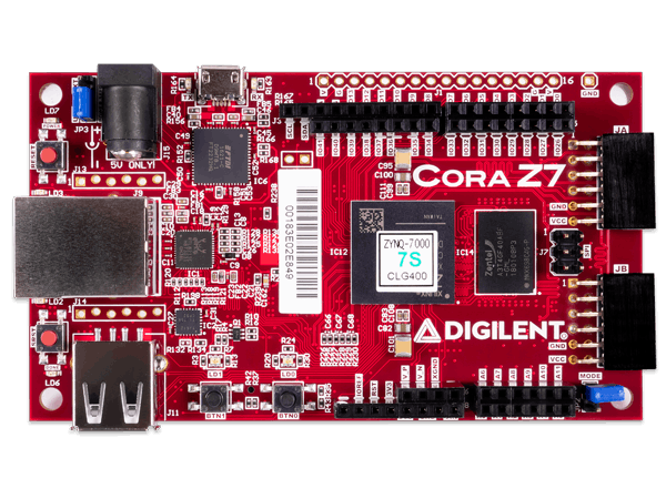
FPGAs can process data very quickly. In order to show how quickly, I decided to compare the speed at which a Pi Estimation algorithm runs in FPGA hardware to how fast the same algorithm runs on a processor. The Cora Z7 is a cheap FPGA development board featuring a Zynq chip - which contains both a processor and FPGA fabric. In a previous project, I took a look at how fast a Monte Carlo Pi Estimation algorithm runs in a Linux OS running on the Cora's processor. Results differed depending on which variant of the Cora was used, since the two variants have different numbers of processor cores, but I am confident that we can blow those numbers out of the water with the speed and parallelism of the FPGA fabric.

This Wikipedia article describes the Monte Carlo method, including a good visualization of how it is used to estimate Pi. Of particular interest to us is the fact that no iteration of the Monte Carlo method depends on the result of another iteration. By this I mean that every test is totally independent of each other test, they can in theory all be done simultaneously. In reality, we cannot do more things simultaneously than the hardware we are using supports, but this means that the Monte Carlo method is a pretty good benchmark to use to see how fast a piece of hardware can process things in parallel.

Vivado Projects

Source code for this project is available in the two repositories linked in the Attachments section. In order to open one of these projects in Vivado, first clone the appropriate repo (each targets a different variant of the Cora) in a console shell - Git Bash is recommended on Windows - using the command below, replacing <REPO URL> as appropriate.

git clone --recursive <REPO URL>

Check out the Vivado project the repo describes by calling the checkout subcommand of the git_vivado.py script in the digilent_vivado_scripts subdirectory with Python 3.

python3 <REPO PATH>/digilent_vivado_scripts/git_vivado.py checkout

Open the XPR file this creates in the proj subdirectory of the repository in Vivado 2018.2. The source code and block design can be looked at and changed using the Vivado IP Integrator's Diagram and Sources panes.

Generate a bitstream. Export hardware and launch Xilinx SDK. In SDK create a new application project and copy-paste all of the files from the sdk/appsrc subdirectory of the repo into the project's src subfolder. From Xilinx SDK, the Cora can be programmed and the SDK project can be run on the Zynq processor. A serial terminal console (like TeraTerm) should be used to view the Zynq processor's print messages, which prints over UART using a baud rate of 115200.

If this section isn't clear, take a look at this tutorial from Digilent for a walk-through of how to use Vivado's IP Integrator and Xilinx SDK.

Estimating Pi in Hardware

The pseudo-code below describes the process required to generate and test a particular sample using the Monte Carlo method of estimating Pi:

x, y = rand()
radius_squared = x*x + y*y
result = (radius_squared < MAX_RADIUS_SQUARED)

The FPGA fabric contained in the Cora's Zynq chip, contains elements called digital signal processing (DSP) slices. These DSPs are used to do certain operations that would otherwise take up too much of the FPGA fabric. In the case of running the Monte Carlo method, we need to do two multiplication operations (x*x and y*y). As long as the result of each multiplication operation is less than 48 bits wide, we only need to use two of the Cora's DSP slices per instance of the code running the Monte Carlo simulation.

I created an AXI module to process a random 32-bit sample (16 bits for x and 16 bits for y) using the Monte Carlo method every clock cycle. This module is described by the AXI_Piestimator.v, piEstimator.v, circleChecker.v, lfsr32.v, and result_accumulator.v files found in the src/hdl subdirectories of the two Github repositories linked in the Attachments section of this project. The Cora Z7-10 has 80 DSP slices, while the Cora Z7-07S only has 66. This means that, since each PiEstimator instance requires two DSP slices, the Z7-10 and Z7-07S can use 40 and 33 PiEstimator instances, respectively. A TCL script, entitled addPiEstimators.tcl, is provided below. This script adds as many PiEstimator instances as possible to a block design when run in a Vivado Project TCL Console.

Random samples are created by using a linear feedback shift register (LFSR), with a seed value provided by the controller. This Wikipedia article describes how LFSRs work.

The result of each sample is added to a running sum in the result_accumulator module. The final result is provided to the controller.

Each PiEstimator instance has an enable pin, and runs as long as enable is held high. The LFSR seed is set and the results are provided back to the Zynq processor via an AXI bus.

I clocked the entire system at 125MHz - increasing or decreasing the clock speed directly affects the performance. I could probably have run the system faster than this, but the PiEstimator module may not have still met timing.

Controlling the Estimators

Since we are working with a potentially large number of PiEstimator instances, and we need to know how long each of them run for, a controller block is needed. This controller is implemented in the AXI_PiEstimator_Control.v and ctrl.v files in the two repositories linked below. It accepts a "duration" value from the Zynq processor over an AXI bus, and allows the Zynq processor to start all of the PiEstimator instances simultaneously. After the shared enable pin has gone low, and the accumulated results of each PiEstimator's simulations is valid, each instance asserts a done signal, which is checked by the processor. The processor then runs through the each instance's result and sums them all up. This sum, multiplied by 4, and divided by the total number of samples (duration multiplied by the number of instances), is an estimate for Pi.

I chose to run as many samples as I could fit in a 32-bit integer. As such, I provided the controller block with a duration of (2^32-1)/N, where N is the number of PiEstimator instances in the project.

Results

See the results printed by each Cora variant pasted below:

Cora Z7-07S:

Utilization:           33 Estimator IPs
                       66 DSP Slices
Elapsed time:          0x07c1f07c clock cycles
                       1.041204 seconds
Samples within circle: 0xc90e9161 samples
Total samples:         0xfffffffc samples
Estimate of pi:        3.141514
Accuracy:              -0.002499 percent

Cora Z7-10:

Utilization:           40 Estimator IPs
                       80 DSP Slices
Elapsed time:          0x06666666 clock cycles
                       0.858993 seconds
Samples within circle: 0xc90e8ea4 samples
Total samples:         0xfffffff0 samples
Estimate of pi:        3.141514
Accuracy:              -0.002519 percent

When we compare these results to the results of the same algorithm run in Linux on the Cora's Zynq processor (see this project), we can a stark difference. Where the slower of the two Cora variants was able to process a full integer's worth of samples in about a second, the faster of the two only managed 100, 000, 000 samples in 1.8 seconds in Linux. In other words, the hardware-accelerated version of the algorithm was 77 times faster.

Conclusion

Hardware is fast, crazy fast. Unfortunately, it can be finicky to work with, and not every algorithm is as easy to parallelize as the Monte Carlo method. If you have any questions, feel free to leave a comment!