Over-engineered dual core light barrier

Simple or complicated?

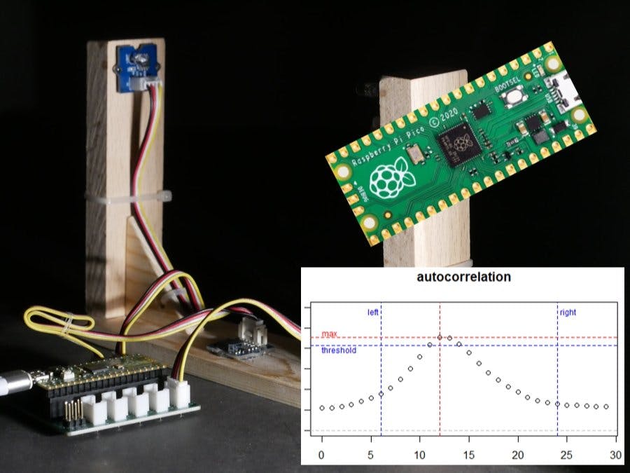
How difficult can it be to build a light barrier? All you need is an LED, a light sensor and some lines of code:

while True:
    measure()
    if not autocorrelation():
        beep(800)

measure() measures the received light that was emitted by the LED. autocorrelation() does a little math to find the signal from the LED in the measured data. And if the signal was not found, then beep() gives an acoustic signal.

Looks simple, doesn't it? But in fact, what's behind these functions is a bit more complicated. Let's go deeper, but before we do, let's take a look at why a light barrier with visible light is more complicated than you might first think:

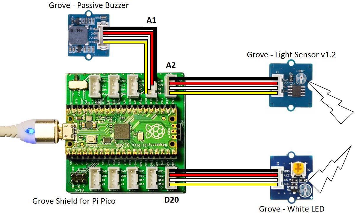
Problem: Ambient light

The setup is very simple: we just connect the light sensor and the LED to the Grove Shield:

And everything can be built with simple materials from the hobby basement:

Now we just need a few lines of code to turn on the LED and read the values of the light sensor continuously. A high value measured with the light sensor indicates a clear view from the LED to the sensor. If the measured value is low, then the light barrier is blocked:

But, unfortunately, such a setup will only work in dark rooms. As soon as light from a lamp falls on the sensor, the sensor permanently measures a high value, so that the value no longer becomes low when the light barrier is blocked:

This makes it very difficult to find the right threshold for the measured light intensity. In addition, most light sources do not emit constant light, but pulses or wave forms:

A simple threshold method will not work here. So we have to be smarter about it.

Solution: Pulsed LED light

Of course, instead of the white LED, you could use an infrared LED and a corresponding IR sensor. That would minimize the problem with ambient light. But that would be too easy. Let's find a solution for a light barrier with visible light.

Instead of turning the LED on permanently, we can pulse it. Then the measured signal looks like this:

This already looks quite promising. But still the ambient light causes problems because the shape of the measured signal changes:

But even with ambient light, the pulsed signal can be easily recognized within the measured data! At least with the human eye. So we only need to write an algorithm, which is able to detect the emitted LED signal in the measured data.

Autocorrelation

You wonder what this is? On the internet you can find the following definition:

Autocorrelation is a mathematical representation of the degree of similarity between a given time series and a lagged version of itself over successive time intervals.

This sounds very mathematical, but it also sounds very promising for our problem. So how does it work?

Let us assume that the LED emits a short single light pulse. This light pulse is measured by the light sensor. Of course, the signal measured by the sensor is noisy and shows an offset:

The duration of the LED signal is shorter than the time during which the data is measured by the light sensor. This allows us to shift the LED signal in time against the measured signal. And during each shift step we multiply the values of the LED signal with the values at the corresponding positions of the measured signal. The sum of these multiplications is then the correlation value for the shift step:

On the left side of the animation you can see the LED signal, which is shifted over the measured data. On the right you can see the calculated correlation value for each shift step.

If a maximum is found in the autocorrelation data, it means that the LED signal was found in the measured data:

At ideal conditions, a simple pulse would be sufficient. But we are dealing with ambient light, which can have a waveform. Then a single pulse from the LED is not clever:

In this example, the light barrier was blocked. This means that no light from the LED reaches the sensor. Nevertheless, the autocorrelation results in a maximum because the background light has a waveform:

Barker-Codes

What we need is a smart pulse pattern for the LED, which gives us an clear result in the autocorrelation.

Fortunately, we do not need to reinvent this, because R. H. Barker developed exactly such codes for telecommunication and radar technology in 1953. These so-called Barker codes are available in different lengths:

If we let the LED flash with such pulse sequences, then we can achieve the most optimal detection result with the autocorrelation:

Code

Now we have everything we need to build a good light barrier. Enough with the theory, now it's time for coding.

The Raspberry Pi Pico has two cores that run independently. This is useful, because then we can use one core to drive the LED with the Barker code sequences and the second core to measure the data from the light sensor. Simultaneous!

To control the LED in a separate core, and consequently also in a separate thread, a own function must be defined for that:

def led_task():
    led.value(False)
    led_start_ticks_us = utime.ticks_us()
    # wait two pulse lenghts before start sequence
    wait_until_ticks(led_start_ticks_us, 2*pulse_length*dt_samples)
    for n, led_on_off in enumerate(Barker_Code):
        if led_on_off > 0:
            led.value(True)
        else:
            led.value(False)
        wait_until_ticks(led_start_ticks_us, (n+3)*pulse_length*dt_samples)
    led.value(False)

With a simple call, this function can then be started as a separate thread:

_thread.start_new_thread(led_task, ())

Because the function is executed on the second core, it runs in parallel to the functions that are executed on the first core. Exactly what we need to measure the sensor data. With this, the measure() function looks like this:

def measure():
    # start the led pulse generation on the second core
    _thread.start_new_thread(led_task, ())
    start_ticks_us = utime.ticks_us()
    for n in range(n_samples):
        data[n] = light_sensor.read_u16() / 0xFFFF
        wait_until_ticks(start_ticks_us, (n+1)*dt_samples)

The function first start the LED-thread and then stores the measured data in the array data[] to later perform the autocorrelation with the LED signal. The LED signal sequence is predefined in the array Barker_Code_samples[]. The autocorrelation() function performs the calculations and stores the correlation values in the array autocorr[]:

def autocorrelation():
    for shift in range(n_autocorr):
        autocorr[shift] = 0
        for pos in range(n_Barker_Code_samples):
            autocorr[shift] += Barker_Code_samples[pos] * data[pos+shift]

And as a result, we get such values when the light of the LED is well to measure:

But how can we detect the maximum in the data? I would say: This is a task for a statemachine:

In state 1, the state machine expects increasing values and waits until the value exceeds a threshold and then waits until the value decreases again. Then the state machine jumps to state 2, where it waits until the value falls below a threshold. Only if this is given, the variable signal_detected is set to True. The following image shows the process using real data:

By using this state machine, the function autocorrelation() will finally look like this:

def autocorrelation():
    autocorr_threshold = 0.75
    autocorr_max = -1000
    autocorr_max_pos = 0
    detection_state = 1
    signal_detected = False
    for shift in range(n_autocorr):
        autocorr[shift] = 0
        for pos in range(n_Barker_Code_samples):
            autocorr[shift] += Barker_Code_samples[pos] * data[pos+shift]
        if detection_state == 1:    
            if autocorr[shift] > autocorr_max:
                autocorr_max = autocorr[shift]
                autocorr_max_pos = shift
            if (autocorr[shift] < autocorr_max) and ((autocorr_max - autocorr[0]) > autocorr_threshold) and (autocorr_max_pos >= autocorr_valid_window[0]):
                if autocorr_max_pos > autocorr_valid_window[1]:
                    detection_state = 3
                else:
                    detection_state = 2
        if detection_state == 2:
            if (autocorr[shift] < (autocorr_max - autocorr_threshold)):
                signal_detected = True
                detection_state = 3
    return (signal_detected)

The function additionally checks whether the maximum lies within the middle area of the shift range. It must not lie at the edges. If a valid maximum was found, then True is returned. Otherwise False.

And that's it: The light barrier is ready!

Here are a few examples where a signal was detected or not detected:

You could have just bought a ready-made light barrier, but then it wouldn't have been as much fun.

Tips and hints

The LED board (Grove - White LED) has a potentiometer with which you can adjust the brightness of the LED. With a brighter LED the light barrier runs more stable but be careful: The LED should not get damaged.

Ambient light is bad for the light barrier, because the light sensor (Grove - Light Sensor v1.2) quickly becomes saturated. This means that the sensor only outputs maximum values. Then a hardware tweak in the form of a small cardboard roll that you put over the sensor helps.

I realized the project with the Grove Starter Kit for Raspberry Pi Pico from Seeed Studio. Instructions on how to install Thonny and set it up for the Raspberry Pi Pico can be found here.

The Raspberry Pico board does not have a reset button. This is a bit annoying, especially when developing multicore applications, because you have to reset the board more often. Therefore I used a magnetic USB cable. This is super easy to disconnect and reconnect.

I developed the project with version v1.19.1 on 2022-06-18 of MicroPython. It may be that the multicore functionality does not (yet) work so well in other versions. Instructions for installing the firmware are available here.

If you want to save the program on the Raspberry Pi Pico so that it is executed automatically as soon as the Pico is supplied with voltage, then you can save the code under the name boot.py on the board. You can find a tutorial here.

Addendum

I hope you enjoyed this project as much as I did. Technically it is nonsense to build a light barrier with a white LED and a light sensor, but it was a challenge to get the best performance out of this setup.

There is much more to the Barker codes than I wrote in the story. But that would have gone beyond the scope. But one thing should be mentioned: The Barker codes are not pulses between 0 and 1 but between -1 and +1. This has considerable advantages in analog technology (Radio signals, Radar, Spread Spectrum). But in our setup it makes almost no difference, because the LED can only be ON or OFF. A negative light signal is not possible ;-).

The actual code is a little more complicated than I described in the story. But the code should be so well documented that the additional details are more or less self-explanatory. Feel free to message me here if you have questions or comments.

In the Github repository is a second version of the code which contains command line output to view the values and an export function to save the data to CSV files for later analysis.

Regards,

Hans-Günther