Autonomous Drone Landing

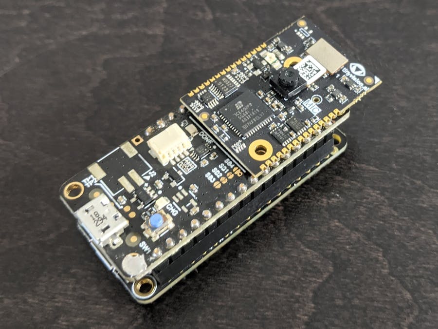
I've spent the last several years at StreamLogic developing tools that aim to make it easier to build and deploy computer vision at the edge. One of my favorite platforms that we target is this Vision FPGA SoM from tinyVision.ai:

Pretty tiny right? At the center you can see a small, low-power, and inexpensive camera module from HiMax Imaging. I'm always on the lookout for new applications that I might target with this platform.

Several months ago, I got exited about drones after a business partner had mentioned one of their agricultural uses cases that used a drone. Drones are a great use case for tinyML; they need a lot of sensor data, and are sensitive to size, weight and power. I knew pretty much nothing about drones, but I spent the weekend trying to get oriented and researching open-source drones. Before the weekend was out, I had purchased a drone: the QAV250 Kit from Holybro.

This drone is not pre-assembled and being a novice, a number of months past before I had all the right parts and got it off the ground. But let's jump to the end of the story. Once I got to actually flying the drone, I realized how inaccurate GPS positioning can be. When flying autonomous missions with autopilot, you may find your drone a good ways away from the planned flight path. This can be pretty hazardous both in flight and landing. That's when I came up with the idea for this project.

The goal is pretty simple: safely land the drone with autopilot. There are two parts to this 1) land on the intended surface (pavement in my case) and 2) avoid any unexpected obstacles on the surface. To accomplish this, I came up with a computer-vision algorithm to detect when and in which direction the drone should move as it lands.

Algorithm Design

My solution is pretty simple at a high level. A downward facing camera is attached to the underside of the drone. It captures images for analysis as the drone slowly descends for landing. First, the square meter directly under the drone is identified and rated as landing site. Second, nearby sites in the eight directions (North, North-East, East, South-East, South, South-West, West, North-West) are also rated. Finally, if any of the nearby sites are rated significantly better than the current site then the drone's position is adjusted in the corresponding direction.

This is an example image taken from my drone:

The black square in the middle is the current landing site if we continue on course. The labeled squares around it are the candidate sites to evaluate for possible changes of direction. Obviously we want to move South-East in this case if we are to land on pavement.

Well, that's the high level, but you may still be wondering 1) how do you know the size of a meter and 2) how do you rate it? The first one is easy, the drone will already have an altitude sensor on board, so you can get an estimate of the height of the drone. Given the height, some camera specs and a little algebra, it's pretty straight forward to calculate the number of pixels per meter (PPM) for the current image. In this case, it works out to PPM = 168 / H.

For the second problem, that's where computer vision comes in. We need to be able to take any arbitrary crop of the image and get a quantitative score as to how likely that image is of unobstructed pavement. The actual value is not that important here, as long as we can compare two scores to determine which is better. One could hand-craft an algorithm, but I choose to train a convolution neural-network (CNN) to generate scores.

The next section will discuss how I trained the CNN, but let's look at the output for the image above:

This graph shows the score for the the current landing site (labeled C) and the candidate sites in all 8 directions. No question here that South-East is the winner as hoped.

Machine Learning

As described above, I chose to use a CNN to generate quantitative scores for candidate landing sites. Specifically, a fully-convolutional network (FCN). These are different than other CNNs in that they do not end with a dense or global pooling layer. The activation maps of the last convolution layer is the network output. As you will see, this works out nicely for this application.

There are different approaches to training a FCN, but I chose to first build a classifier CNN and then convert that to a FCN. Let's start by looking at how I built the classifier.

I wanted to create a classifier that would classify small image patches as good or bad. But first, I need data. Naturally, I spent a good amount of time searching the Internet for some public datasets. Unfortunately, nothing really fit the bill for my task. I needed to create my own dataset, but how? In the end, I created my own Battery-powered Image Logger.

The image logger captures images every second and writes them to an SD card. This gave me the ability to collect images from my drone during landing like this one:

With a number of images in hand, I created a dataset of patches in three different categories:

• ground (not pavement)
• pavement
• unknown (edge of pavement/not pavement)

I initially collected around 2, 000 patches. I then spend a good deal of time trying to train a shallow network (2 convolutional layers) without much success. I tried a number of data augmentations and network structures to no avail. The network would always generate random results on the validation set or make a constant choice (:sigh:).

There was nothing left to do but get more data. So, I collected about another 1, 800 patches from my images. Bingo, with around 4, 800 patches, training was behaving, and after a little experimentation, I had a network that achieved 88% accuracy. Here is the final network:

model = Sequential([
    layers.Input(shape=(tgt_width,tgt_height,3)),
    layers.Conv2D(10, 5, strides=2, padding='valid', activation='relu'),
    layers.Conv2D(3, 3, padding='valid'),
    layers.GlobalAveragePooling2D(),
])

This model has only 1, 033 parameters!

For the complete training procedure see the training.ipynb Jupyter notebook in the code repository.

Fully-Convolutional Network

With a ground patch classifier in hand, it's time to convert that into a FCN that we can apply to the whole image. Looking at the network above, you can see that by removing the GlobalAveragePooling2D layer, we end up with a network that contains only convolution layers. It accepts any image size and produces an activation map of proportional size. The result of the FCN is effectively the same as applying the patch classifier over all patches in the image in a sliding-window fashion. The activation value at each location in the output map is the classifier result for the patch at the corresponding location in the input image.

Does that really work? Let's have a look. Here's a rendering of an example image and the corresponding output of the FCN:

The right image is showing the FCN output for the pavement class. Summing the values in the right image over a candidate sites gives us the score for that site.

Here's another way to render the same data:

In this image, I overlaid the original image with a red square whose transparency is the inverse of the output for the pavement class (i.e. the more likely it is pavement, the more transparent). Looking at the target landing sites, the more red there is, the lower the score.

All the details for creating the FCN and transferring the weights from the trained classifier to the FCN are in the evaluation.ipynb Python notebook in the code repository.

Quantization

I quantized the network to use 8-bit weights and 8-bit activations for better run-time performance. You could follow the standard procedure described in the Tensorflow documentation, but I used my own approach which has a simpler quantization model. The procedure is detailed in the README of the code repository.

Here's an example of the output from the quantized network:

This is nearly indistinguishable from the output from the original network:

Hardware Build

I already had a hardware stack with the Vision FPGA SoM and a microcontroller from the Battery-powered Image Logger project. Unfortunately, the microcontroller turned out to be too small. Calculating the size of the input/output activation maps of each layer in the FCN, we find that we need 48KB of buffer space. Fortunately, there is another Feather board that fits the bill.

The Feather M4 Express is not only faster, but it has a whopping 192KB of RAM! We don't need an SD card for this project, so our build is just the Vision FPGA SoM board stacked on the Feather M4 Express.

Small, lightweight and battery powered!

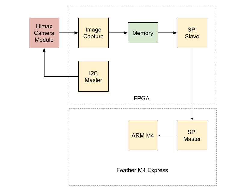
Implementation

From the block diagram you can see the FPGA is used as bridge between the camera module and the microcontroller.

The FPGA passes the captured image to the microcontroller in the raw format of the image sensor which is a Bayer filter image. The pre-built programming file for the FPGA is provided in the code repository.

That leaves the microcontroller with the task of:

• Converting the image from Bayer to RGB format
• Downsampling the image to 80x80
• Performing the FCN inference
• Summing the target site regions

The source code for all these tasks is included in the sketch folder of the code repository. I'll make just a few comments about the code here.

The complete raw image is over 100KB, and although this MCU has 192KB, I don't want to waste space unnecessarily. The downsampled image only requires 20KB. You will see in the loop that reads the image from the FPGA that it performs the Bayer conversion and downsampling while it's reading, one block at a time, so we only need enough space for the downsampled image.

Instead of using a CNN framework, this network is so simple that I implemented my own convolution and activation functions. Those are defined in the gndnet.cpp file. It's written in a pretty straight forward manner, if you are interested in learning more about how convolution works. I wasn't worried too much about performance, but these could probably be replaced by functions from ARM's neural network library for better performance.

Results

Integration of the landing algorithm with the drone's flight controller was out of scope for this proof-of-concept. The goal was to design and train the algorithm, demonstrate it's effectiveness and obtain some performance data.

Qualitatively the algorithm looks good. It's been evaluated on test images from the site used for training and also sites not used for training. The results have been very encouraging. Of course, to go to production, one would want to train on data from more than one site.

In terms of performance, the whole process from image capture to score calculation is a around 525 ms. That means a little less than 2 FPS. That would probably work as the drone does descend at a fairly slow pace. However, this can easily be improved. For example, if the Bayer conversion and downsampling functionality was moved to the FPGA, that would bring the time down to a little over 200 ms. That would over 4 FPS, which is definitely sufficient.