


Hardware components | ||||||
 |
| × | 1 | |||
| × | 1 | ||||
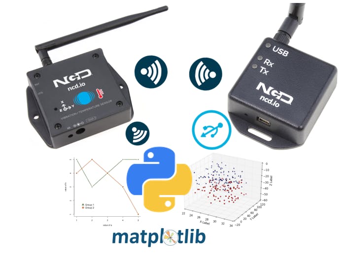
In this blogtut, We are going to plot Live streaming graph which helps us to monitor the data of wireless vibration sensor after a certain interval of time.
Hardware Used- Python
- XCTU — Digi Mesh Software
- Matplotlib
- Serial
- Mpl_toolkits
- Matplotlib animation
The dual power backup mode Wireless Vibration sensor has the capability to monitor the real-time parameters of vibration sensed from many high tech machines and can be used in various different applications. You can also use the sensor with 2AA batteries which allows the Wireless sensor to transmit 500, 000 parameter transmission at a time. We can also transmit the data to the gateway device for 10 years maximum with 2AA battery backup by following some certain interval conditions.
ApplicationIn this application, we are plotting the two dimensional(2D) and three-dimensional(3D) graph by fetching the RMS(in X, Y, Z axis) values from the sensor wirelessly. The graph plotting the values continuously after a certain interval of time. The live streaming on 2D and 3D has various uses but for the basic start, we have used this sensor with the industrial machines to sense the vibration parameters at 2D as well as a 3D axis.
Wireless and Serial CommunicationTo fetch the parameters we are using the Xbee coordinator which receives the values of Wireless Vibration Sensor through wireless communication.
Install PythonTo install the python we just have to go the link and install the version as per your requirement. After Installing the python
- Click on Command prompt
- Install the Pyserial,Matplotlib,Numpy packages, all the packages will be used in this project
After installing all the packages we are going to connect the Xbee coordinator and with the help of the reference link, we will adjust the parameters of the Wireless Vibration Sensor to fetch the byte array from the device.
About CodeAfter the Adjustment, we will use the serial code which helps us to manipulate the byte array which is mentioned in the manual of the sensor and share the parameters as per the requirement.
- Import the Serial package
import serial
- Mention the serial port and baud rate through which you want to read the Byte Array.
seru = serial.Serial('COM6', 115200)
- If the serial port is true then we will continuously read the byte array from the Wireless Vibration sensor through xbee coordinator connected serially to laptop port
while True: s = seru.read(54)
Note: In this sensor, we are fetching 54 bytes in one go which is mentioned in the manual you can mention the byte array which is given in per the sensor manual
- Going through some certain manipulation we were able to manipulate the data as per the requirements
print('Sensor Number: '+str(s[16]))
print('Firmware No: '+str(s[17]))
rms_x = (((s[24]*65536)+(s[25]*256)+s[26])& 0xffff)/100
rms_y = (((s[27]*65536)+(s[28]*256)+s[29])& 0xffff)/100
rms_z = (((s[30]*65536)+(s[31]*256)+s[32])& 0xffff)/100
print('RMS X axis: '+(str(rms_x))+' mg')
print('RMS Y axis: '+(str(rms_y))+' mg')
print('RMS z axis: '+(str(rms_z))+' mg')
max_x = (((s[33]* 65536)+(s[34]*256)+s[35])& 0xffff)/100
max_y = (((s[36]*65536)+(s[37]*256)+s[38])& 0xffff)/100
max_z = (((s[39]*65536)+(s[40]*256)+s[41])& 0xffff)/100
print('Max Value X axis: '+(str(max_x))+' mg')
print('Max Value Y axis: '+(str(max_y))+' mg')
print('Max Value Z axis: '+(str(max_z))+' mg')
min_x = (((s[42]*65536)+(s[43]*256)+s[44])& 0xffff)/100
min_y = (((s[45]*65536)+(s[46]*256)+s[47])& 0xffff)/100
min_z = (((s[48]*65536)+(s[49]*256)+s[50])& 0xffff)/100
print('Min Value X axis: '+(str(min_x))+' mg')
print('Min Value Y axis: '+(str(min_y))+' mg')
print('Min Value Z axis: '+(str(min_z))+' mg')
ctemp = (((s[51]*256)+s[52])& 0xffff)
battery = ((s[18]*256)+s[19])
voltage = 0.00322*battery
print('Temperature in Celcius: '+(str(ctemp)))
print('ADC Value: '+(str(battery)))
print('Battrey Voltage: '+(str(voltage)))
Going through the image we will be able to monitor the sensor parameters from the python shell.
2D and 3D live Graph Plotting
for 2D and 3D graph plotting we have installed the package called Numpy and Matplotlib which plays a significant role in creating the plot
For plotting the graph basically, we will be using matplotlib and to continue streaming the data for which we will be using the Animation function within the matplotlib
- Importing matplotlib library
import matplotlib.pyplot as pltimport matplotlib.animation as animation
- Create the function of serial code for wireless vibration sensor and return the value values which you want to display in graph plot from the functions
- Create a figure for Plotting
fig = plt.figure()ax1 = fig.add_subplot(1,1,1)
- Assign the values globally and append the Vibration sensor function values with another function which helps to animate and plot the graph
rmsX,rmsY,rmsZ = vib_sense();
xs.append(dt.datetime.now().strftime('%H:%M:%S.%f'))
ys.append(rmsX)
y2.append(rmsY)
y3.append(rmsZ)
- Limit the Sensor data axis notation
xs = xs[-50:]ys = ys[-50:]y2 = y2[-50:]y3 = y3[-50:]
- Mention the commands which help you to Plot the graph in different styles
ax1.clear()
ax1.plot(xs, ys, label='RMS X', marker='o')
ax1.plot(xs, y2, label='RMS Y',marker='o')
ax1.plot(xs, y3, label='RMS Z',marker='o')
- Initializing the animation function will help to animate the sensor data on plotting the graph
ani = animation.FuncAnimation(fig, animate, fargs=(xs, ys, y2, y3), interval=500)plt.show()
Note: The only thing which is different between plotting 3D graph is that we have to use the numpy.array which has grid values which are all of the same types and has been indexed by a tuple function, you can also learn about from reference Link. And a figure for plotting will be mentioned as
ax = fig.add_subplot(111, projection='3d')
- for the 3D graphing we will use the numpy.array function in which we will create the plotting function accordingly which represent the data the in wireframe style or scatter style
def update_lines(num):
#calling sensor function
rmsX,rmsY,rmsZ = vib_sense()
#Creating Numpy array and appending the values
vib_x= np.array(rmsX)
x.append(vib_x)
vib_y= np.array(rmsY)
y.append(vib_y)
vib_z= np.array(rmsZ)
z.append(vib_z)
print(x)
print(y)
print(z)
ax = fig.add_subplot(111, projection='3d')
ax.clear()
#Limit the Graph
ax.set_xlim3d(0, 100)
ax.set_ylim3d(0, 100)
ax.set_zlim3d(0, 100)
#for line graph
graph = ax.plot3D(x,y,z,color='orange',marker='o')

#For Scatter
# graph = ax.scatter3D(x,y,z,color='orange',marker='o')
return graph
- Python forums
- Matplotlib Tutorials
- Numpy tutorials
- Pyserial


Comments