Synthesize music with animations on a Raspberry Pi Pico

Follow the Arm Software Developers team for more resources like this ! X: @ArmSoftwareDev and YouTube: Arm Software Developers .

Introduction

The Raspberry Pi Pico is an extremely popular and capable MCU (microcontroller) development platform that is based on Raspberry Pi's RP2040 MCU and costs only $4. The RP2040 incorporates two 133 MHz Arm's Cortex-M0+ CPU cores, 264 kB of SRAM and a unique programmable I/O system.

This guide will walk through the integration of several software components to create a MIDI player with spectrum visualization and animations. I will explore how we can create a complex software, with real-time audio synthesis, visualization and dual-core without using an RTOS.

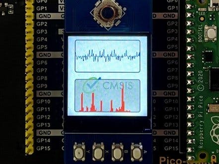
You can see and listen to a preview of the result below:

The audio will be generated using the PWM audio driver from the pico-extras and the LCD will be controlled with the LCD driver from the PIO pico-examples (modified for the demo).

The software components will be integrated using the CMSIS-Stream open source library.

MIDI components come from the Playtune Synth project by Len Shustek and have been modified a lot to be integrated in this demo.

The demo uses the two M0+ cores.

Data flow and CMSIS-Stream

This demo uses several software components that come from different origins:

• Some software developed by Raspberry: PWM driver and LCD driver.
• Some components from the Playsynth_tune project by Len Shustek for the music synthesis
• CMSIS-DSP components for the signal processing (spectrum computation)
• Application specific components developed for this demo
• Arm-2D for the final display

Those components must be connected to achieve the desired outcome: real-time music synthesis with animated display.

With streaming applications, it is quite useful to represent the software architecture as a graph that highlights the data flow and the data dependencies.

There are two graphs:

• One on core 0 to synthesize the music: the Audio graph.

• One on core 1 to process and display the music: the LCD graph.

(Higher resolution pictures of the graphs can be seen on the project's github)

There are several problems to solve to implement those graphs:

• Different parts of the graph use different data rates. For instance, the LCD refresh rate is smaller than the audio rate. Therefore, some nodes in the graph must be executed much less often than other nodes. How do we do that easily without an RTOS ?
• Because of the different data rates and because some nodes work on buffers of different sizes, there is the need to introduce FIFOs between the nodes. How do we size those FIFOs ?
• When nodes work on buffers of same size, we still need temporary buffers between those nodes: how do we minimize the temporary memory that is used to execute the graph ?
• How do we integrate software components in such a system: connection to the FIFO etc … but with minimum effort from the developer

All those problems can be solved manually. They are not so difficult. But they add friction in the development flow. As a developer you must think about all of these details instead of focusing on what is the real added value of the product.

Also, those problems make the software less modular: any change in the graph (data rate, buffer size consumed or produced by a component) may impact the scheduling of the whole graph and the sizing of lots of FIFOs. It makes the life of the developer more difficult if each time something is changed, all those graph scheduling details must be considered and modified again.

CMSIS-Stream has been developed to make the life of the developer easier by handling all those details:

The graphs are described in Python.

CMSIS-Stream computes a static schedule at build time from the Python description:

• It is a periodic sequence of function calls that will generate / process a stream of samples considering the different data rates and buffer sizes.

CMSIS-Stream sizes the FIFOs considering the computed schedule and the size of buffer consumed or produced by the nodes.

CMSIS-Stream tries to minimize the temporary memory used by the buffers.

The software components are integrated in the graph:

• Directly if they are just pure functions.
• With a very light C++ wrapper that provides standard raw pointers to the components to access the FIFO

The graphs are described in the python scripts create_audio_graph.py and create_lcd_graph.py.

Please refer to the CMSIS-Stream documentation if you want to understand how to use CMSIS-Stream and change the graphs.

The audio graph

The audio graph is mainly made from components coming from the Playsynth_tune project by Len Shustek. But they have been modified a lot to be integrated in this demo (and bugs were probably introduced).

The fixed point format for the phase increments has been modified to take into account the audio rate used in this demo.

The audio interpolation for the waveform oscillators has been removed: it may be reintroduced later by using the Pico HW interpolator.

The sequencer generating the note commands is part of the graph and not working from an external thread anymore. The logic had to be changed to respect the synchronous behavior of the graph: the output channels of the sequencer must be loaded as much as possible with note commands before the node is finishing its execution for the current iteration of the schedule.

The node sending data to core 1 is not blocking: audio is more important than display. If the LCD graph running on core 1 is too slow, it will just miss a few audio blocks.

The LCD graph

The LCD used for this demo only has a width of 240 pixels. If a refresh rate of 40ms was the target, then it means that only 240 samples would be displayed every 40ms.

But in 40ms much more than 240 audio samples are generated. The audio signal must be filtered and decimated. The LCD graph contains filtering and decimator nodes for the amplitude and spectrum part. The decimation factor is quite high so high frequencies will not be visible on the display.

For the spectrum, one may experiment with bigger FFTs and a smaller decimation factor to try to display higher frequency contents. The advantage of using CMSIS-Stream is that you can easily make those experiments by changing a few parameters in the Python that describes the LCD graph.

You may also need to change the decimation filter coefficients: the coefficients are defined in main.cpp

The spectrum computation is standard:

• The signal is multiplied by a Hanning window.
• It is converted to complex numbers.
• A complex FFT is used.
• The amplitude of the FFT is computed and some scaling (for display) is applied.

The graphic part uses some buffer generators: the buffers are reused between different schedule iterations.

The amplitude and spectrum widgets draw into those buffers. Arm-2D finally composes those buffers using the Pico HW interpolator for blending.

CMSIS-DSP

The open-source compute library CMSIS-DSP is used to do the mixing of the audio channels with a saturating add. It is also used to do the filtering and decimation, to compute the Hanning window and the FFT.

On an M0+, CMSIS-DSP cannot provide any acceleration. But by using CMSIS-DSP you make your software portable to more powerful Cortex processors (M and A) where CMSIS-DSP will provide accelerations for free.

Hardware setup

If you are using a Raspberry Pi Pico board without pre-soldered headers, follow MagPi's "How to solder GPIO pin headers to Raspberry Pi Pico" guide and solder headers to the board.

The LCD is connected through the Pico quad expander so there is nothing else to do.

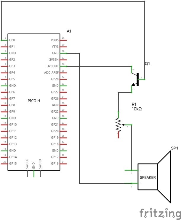
The external speaker must be connected through a transistor otherwise too much current would be drawn from the Pico pin.

Speaker connection

The color coding of the wires is coherent with the photo below. Unfortunately, I had to use what was available at my home and it forced me to use red or purple wires for the ground connection and blue wire for 3V connection.

LCD Connection

The LCD is connected through the Pico quad expander so there is nothing else to do:

Software setup

Setting up the Pico SDK environment

You'll first need to set up your computer with Raspberry Pi's Pico SDK and required toolchains.

See the"Getting started with Raspberry Pi Pico" for more information.

Section 2.1 of the guide can be used for all Operating Systems, followed by the operating specific section:

• Linux: Section 2.2
• macOS: Section 9.1
• Windows: Section 9.2

You’ll need pico-sdk and pico-extras.

Getting and compiling the PicoMusic demo

Make sure the PICO_SDK environment variables are set.

export PICO_SDK_PATH=/path/to/pico-sdk
export PICO_EXTRAS_PATH=/path/to/pico-extras

In a terminal window, clone the git repository and change directories:

cd ~/ 
 
git clone --recurse-submodules https://github.com/christophe0606/PicoMusic.git
 
cd PicoMusic

Create a build directory and change directories to it:

mkdir build.tmp
 
cd build.tmp

Run cmake and make to compile:

cmake -G “Unix Makefiles” -DPICO_BOARD=pico .. 
make

Hold down the BOOTSEL button on the board, while plugging the board into your computer with a USB cable.

Copy the stream.uf2 file to the mounted Raspberry Pi Pico boot disk:

cp -a stream.uf2 /Volumes/RPI-RP2/.

Testing

Just plug your Pico and the demo will start. You can control it with the LCD buttons.

It is also possible to control it from a serial console on your host computer through the USB

Conclusion

This guide covered how you can use a Raspberry Pi Pico board with an LCD and an external speaker to create a real-time music synthesis and spectrogram visualizer. The project uses several components that are integrated in the project using the CMSIS-Stream library.

The Raspberry Pi RP2040's PIO, DMA and HW interpolator were keys to make this demo possible.

You can see the code for the project on the following GitHub repository: https://github.com/christophe0606/PicoMusic

You can learn more about CMSIS-Stream here:

https://github.com/ARM-software/CMSIS-Stream

And CMSIS-DSP here:

https://github.com/ARM-software/CMSIS-DSP