

Hardware components | ||||||
_wzec989qrF.jpg?auto=compress%2Cformat&w=48&h=48&fit=fill&bg=ffffff) |
| × | 1 | |||
Software apps and online services | ||||||
 |
| |||||
This article is about how to model and use the Sharp® IR Sensor (GP2Y0A02YK0F) with Simulink® and Arduino® in a robotics project. The intention is to show how to work with Model-Based Design. For some robotics applications the modeling and filtering used here is overkill. Even if that is the case, it is always good to have some insight into how a system works if something unexpected happens. Choosing the right level of modeling and complexity of a system is an important engineering skill.
In this first part we will focus on modeling the sensor and getting a reliable distance measurement. An advantage with this approach is that it won’t use any CPU time when no obstacle is detected. In the third article we will include the sensor model into a simulation environment for mobile robots. In the fourth and final article we will test all parts on a real robot platform.
Project FilesRequired Hardware- Arduino Mega 2506 board
- Small breadboard with wires
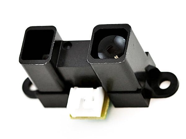
- 1 Sharp IR Sensor GP2Y0A02YK0F
- 1 Capacitor 10uF – 100 uF
- 1 Capacitor 1 uF
- 1 Capacitor 200 nF
- 1 Resistor 10 ohm
In control theory, the combination of sensors, actuators, and elements that process such signals is often referred to as a ‘plant’. Plant models are important and have many purposes. By modeling the system around the parts that will run on the CPU, it’s possible to test a design early and inexpensively. System simulations are very efficient in finding errors without damaging hardware and even in some cases before any hardware is available. System models also allow experimentation with new ideas. For example. with a suitable system model ideas for robot navigation can easily be evaluated. Some can be discarded and some that looks more promising can be further developed.
Plant modeling is a learning opportunity. Knowledge about how the system works is created which can be very useful for development of the software, for debugging and perhaps even more important to get new ideas about how to use it. Plant modeling is a knowledge creating activity and the knowledge is stored in models where other people easily can obtain it.
Fidelity of plant modelsWhat is a suitable plant model? How detailed should it be? Choosing the right level of details is hard. Some developers over-do it and others ignore important behavior. There is a trade-off between accuracy, time spent on modeling (and gaining knowledge) and simulation time. To decide how much effort to use in a specific case is a skill that develops over time with experience. There is no correct answer and system development can benefit from having several plant models with different fidelity. For example a detailed plant model for controller evaluation and one with less details to test logic.
Plant models can be obtained by first-principles or by data driven modeling. The most common way is to use a combination of them. In this article we will use an ad-hoc approach that resembles the learning process.
Task 1 – Checking the sensorThis is the first step in the plant modeling and learning process about the sensor. Connect +5V, GND and the sensor output to analog in 0. Check the datasheet for pin out of the sensor.
Use the Arduino IDE and the sketch below to print sensor readings on the serial monitor.
The values read from the sensor fluctuate quite a lot even with a fixed obstacle in front of the sensor. In my case it varies between 152 and 191. Could this just be sensor noise? Connecting an oscilloscope to the sensor output gives a clue:
With a frequency of 1000 Hz there are peaks on the sensor output of about 90 mV. The sensor sends bursts of infrared lights every millisecond and outputs a voltage level based on which element of the sensor is struck by the reflected light. To read more about how the sensor works look at this article.
It seems like the peaks consists of one fast mode (the initial peak) and one slow mode. There is also some noise on the signal. It is possible to detail this more and dig into the electrical characteristics but something (experience) tells me that this is sufficient for a robotics project.
The datasheet also shows that the output voltage level is non-linear according to the diagram:
From task 1 we learned that there are three components to the output signal of the sensor:
- A nonlinear function from distance to voltage level. The function goes from 0 cm to 150 cm which is the sensor maximum range.
- Measurement noise
- Peaks with fast and slow dynamics
The non-linear function can easily be implemented with a look-up-table in Simulink. Measuring in the figure from the data sheet gives:
table_data = [0 2.3 2.75 2.55 2 1.55 1.25 1.05 0.9 0.8 0.725 0.65 0.6 0.55 0.5 0.495 0.49];
breakpoints = [0 10 15 20 30 40 50 60 70 80 90 100 110 120 130 140 150] / 100;
plot(breakpoints, table_data);
title('Sensor output value');
xlabel('Distance (m)');
ylabel('Voltage (V)');
grid on;
The measurement noise is modeled by Band-Limited White Noise. The power and sample time parameters have to be identified. I did this by testing out different numbers. For sample time I know from the measurement that the peaks are slightly more than 0.1 ms wide and the noise should be faster. A value of 0.1 ms / 125 worked fine. The power was gradually decreased until the Simulink scope showed a similar level of noise as the measurement.
The dynamicsData-driven modeling can now be used to obtain a transfer function for the dynamics using the system identification toolbox. In this case I chose to just add two transfer functions. One first order transfer function for the slow dynamics and one second order for the fast dynamics. A pulse generator will drive the transfer functions.
Based on my measurements, we see that the slow dynamics rises about 30 mV during the pulse. This means that the static gain should be about 0.03. The rise time for a first order function is:
With static gain K = 0.03 we get:
These are good initial values and with some manual tweaking to make the step response look like the measurement I ended up with:
For the second order function we have:
As it should be faster than the first order function I choose f = 100 kHz and xi = 0.7.
Scope output from the slow and fast dynamics:
The components are simply added together and the resulting Simulink model looks like this:
And the simulation output:
Note! Using the oscilloscope to measure the voltage from the sensor for measured distances shows that my sensor gives slightly lower voltage than the table in the data sheet. This can be due to individual differences of sensors and/or the electrical characteristics in the Arduino analog input. Just to be safe, I kept the table values here and if necessary, I can calibrate later.
Task 3 – Smoothing the signalReading the datasheet for the sensor I also found out that it is recommended to use a fairly large capacitor between Vcc and gnd as close to the sensor as possible to limit the peaks during a burst. In addition to the large capacitor I also add a small one of 200 nF to suppress some high frequency noise on the supply voltage.
To further smoothen out the sensor output I add a simple passive filter, an RC-filter.
This filter has a cutoff frequency of:
To filter at least the fast dynamics the cutoff frequency should be lower than 100 kHz. Also it can’t be too low as changes in distance from the sensor would lag. Simulation is an excellent tool to play around with designs like this and see what happens and learn how it works. I choose the cutoff frequency of about 16 kHz after some experimentation. Than means that 2*pi*R*C = 1 / 16000. R should be as low as possible to avoid static error and I found that 10 ohm was available and then C = 1 uF.
Applying the capacitors and the filter and measuring the filtered output I got the result below:
This is the circuit:
To model the effects of the bypass capacitors I simply reduced the amplitude on the pulse generation to 0.1, giving one tenth of the output. I also increased the noise to make it more accurate. The filter is is implemented as a first order filter, RC / (s + RC), see model in the next task. The simulation output now looks like this:
With the model here it is not possible to capture the effect of the bypass capacitors as this would require a more detailed model of the electrical characteristics of the sensor. The approximation by reducing the spikes is sufficient for our robotics application.
It is possible to use SimElectronics to implement this plant model in more detail and in a domain specific manner.
Task 4 – Sample the signalTo use the measured signal in a model that can be executed on an Arduino target, two things have to be supplied; a sample time and the correct datatypes. The Arduino analog input block outputs a 16 bit unsigned integer. In our application we chose a sample time of 100 ms.
Analog to digital conversion with default reference voltage (5V) outputs values between 0 (0V) and 1023 (5V). To convert our measured voltage we need to multiply the signal by 1023 and divide by 5. Before multiplying and adding noise, the continuous signal is sampled at 100 ms. The reason for sampling before is to speed up our simulation. If it was sampled after our modifications, these operations would have to be done a lot more often together with the continuous parts of the model, thus bogging down our simulation.
The gain block doing the multiplication also converts the signal to an unsigned 16-bit integer and saturates the signal to avoid wrapping for negative input voltages. This guards against the case when the input voltage is 0 and the noise is less than 0. Without this saturation, the result would be a very large number.
Note that there is no saturation on the 5V maximum input. In the model, the output would just continue over 1023. On the real board the input pin of the board would probably be damaged. The best approach is to check for over voltage and at least give a simulation warning, but this is left as an exercise. Just adding a saturation block, for example, means that this error condition would not be easily detected by simulation and could cause a hardware failure.
Reading the analog input gives us a value between 0 and 1023 corresponding to 0 V to 5 V. There are many ways to convert this signal to a useful distance. Here I have chosen to use a look-up-table because the distance is nonlinear and a look-up-table is easy to calibrate.
We can now reuse what we learned during modeling of the sensor and sampling. The first step is to invert the look-up-table used for the sensor. This is problematic because the function is not monotonic when inverted. For example, the sensor gives approximately the same output voltage for a distance of 10 cm and 25 cm. To solve this we need to remove the first two values: 0 and 10 cm. The result is that only ranges between 20 and 150 cm could be measured. This is also the operating range of the sensor according to the specifications. This means that if we have an obstacle at 10 cm, the Arduino software will think that it is at 25 cm. This has to be accounted for in the design of the rest of the system. Some ways to account for it are to stop before the minimum range, use another sensor for short ranges or place the sensor at the back of the robot facing forward.
In addition to inverting the table, we need to compensate for the sampling. The break points of the table contain voltages from 0.49 V to 2.75 V, but our read values are integers from 0 to 1023. Multiplying by 5 and dividing by 1023 should give us the correct values. However, that would give us a voltage between 0 and 5 and with integers that would not give sufficient resolution. Therefore we also multiply by 1000 to get the integer value in mV. We do the same thing with the distance and get the output range measurements in millimeters.
Finally, we put in a block that checks for a threshold and outputs 0 if the range is higher than 250 mm or 1 if it is lower. This check will be used to light up the user LED on the Arduino board in the next step.
To further test the model, put in a ramp as the distance and check that the Boolean output triggers at the correct distance.
The inverted table with compensation for the sampling and the breakpoints:
inv_table = uint16([150 140 130 120 110 100 90 80 70 60 50 40 30 20 15]*10);break_points = [490 495 500 550 600 650 725 800 900 1050 1250 1550 2000 2550 2750] * 1023/(5*1000);plot(break_points, inv_table);title('Distance table');ylabel('Distance output (mm)');xlabel('Sampled value');grid on;
The full model now looks like this:
The modeling and high level design of this system is now done. The next step is to clean up the model a bit and design an architecture that allows us to both simulate the full system and run the algorithm on our target hardware. If the Arduino input blocks are connected it is no longer possible to use the plant model. It is also good design to make the actual software implementation platform-independent. Using referenced models we can create three models:
- Full system model (with plant)
- Software model (the algorithm)
- An Arduino platform model, with Arduino I/O blocks
The full system model and the Arduino platform model can now be combined into a Model block, which references both the software and hardware models. This affords us the following:
- Information is only stored in one place, no need to duplicate the software model.
- Platform-independent software model, can easily use it with another target by changing the platform model only.
- Plant and software models are easy to validate and test.
The system model:
And the Arduino subsystem:
Note that software_6 is a separate model, a referenced model:
So to run the software model, the platform model below includes the Arduino I/O blocks and also references the software_6 model.
Load and run the platform_6 model on target with attached sensor, filter and capacitors. Move an object towards and away from the sensor to see when the user LED turns on.
This simple application can now be used to calibrate the look-up-table. Put obstacles at a specific distance, for example 25 cm, and use 250 as the value within the ‘compare block’.. Check if the LED triggers close to 25 cm by moving the object slightly. If it does not light up, adjust the look-up-table’s breakpoints near 25 cm.
Suggested experimentsUsing a look-up-table is just one approach for mapping non-linear functions. Try to come up with an exponential equation matching the function.
Try to check the sensor against different materials such as dark fabric and white paper. Is there a difference?
For some simulations, computation time can be critical. The effect of noise and spikes are not always needed. In such cases it could be beneficial to make a simple plant model by removing everything except the look-up-table. Some ripple in the sampling should be the only difference from a software perspective. The model with higher fidelity can still be used occasionally to check that it works with more details as well. Create these different plant models and compare the software output. How large is the difference?
SummaryThis is a small example that shows some interesting aspects of Model-Based Design. The main takeaway from modeling is knowledge and an understanding of how the sensor works. This knowledge is important when using the sensor in an actual application under different conditions.
In the next article we will implement a new Arduino block that captures the range threshold with an interrupt instead of checking the range on every time step as we did in this article. The advantage of the interrupt approach is that it doesn’t require any CPU execution until the threshold triggers.
Useful links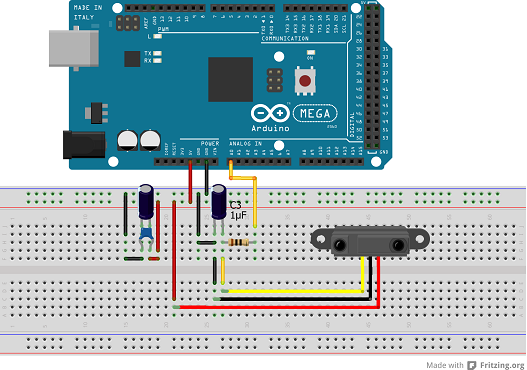


Comments