ME446 Final Showcase: CRS Robot Arm Obstacle Course

Our final project is manipulating a ThermoFisher CRS CataLyst 5 robotic arm to complete a series of tasks, including navigating obstacles, applying force to an egg, and moving to its final position.

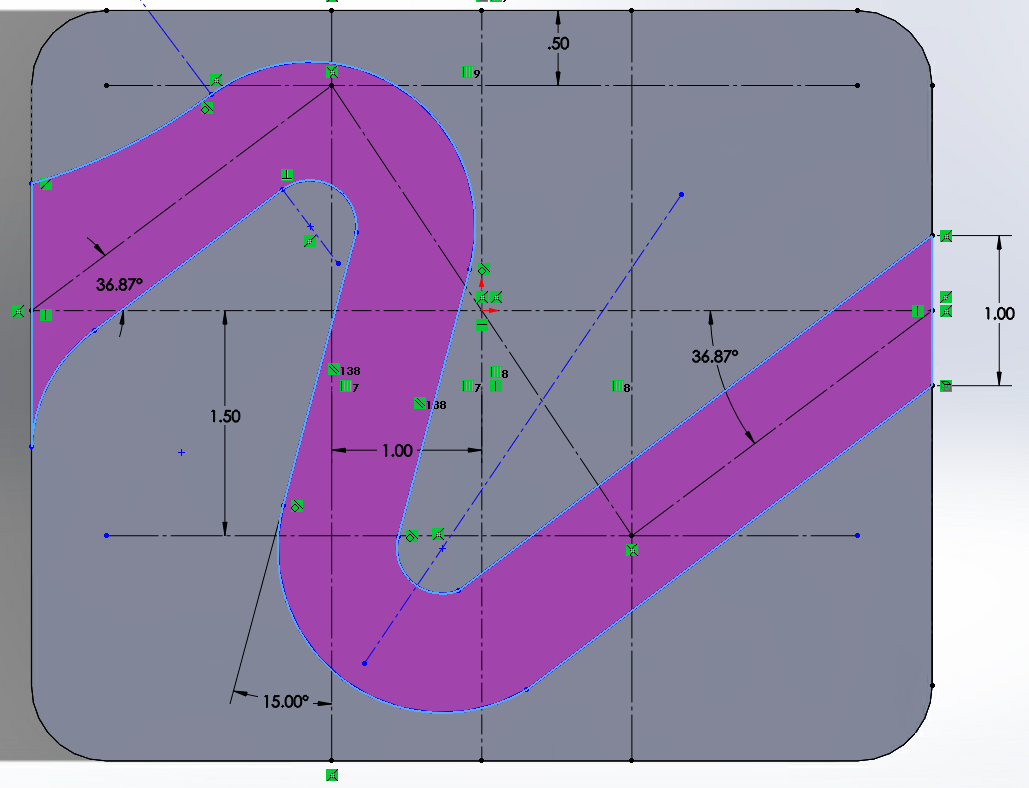
The robot arm uses a combination of straight-line trajectories and coordinated motor movements to complete the tasks. It starts at its resting position, then moves to insert its peg into a to a specified hole before navigating through a zig-zag obstacle course and finishing off with applying force to an egg. The clearances to navigate the obstacle course are on the order of a couple milimeters, which requires careful control over the motors.

The Task

Starting from the robot's resting position, the peg end-effector must reach the following waypoints to complete each task:

• Point 1-2: Move to a position of your choice from the resting position

• Point 2-3: Move the peg just above the hole directly to the left of the robot

• Point 3-4: Insert the peg into the hole and stay for at least 0.5 seconds, then pull it out

• Point 4-5: Navigate around obstacles to bring the peg to the entrance of the zig-zag

• Point 5-7: Navigate through the zig-zag obstacle course, maintaining a certain depth

• Point 7-8: Move the peg just above the egg

• Point 8-9: Push down on the egg with the peg to apply a specific force (500-1, 000 grams) for two seconds

• Point 9-10: Move the robot arm to its final position at (x, y, z)=(10, 0, 20) in.

Development

Task-Space Control

Initially, our focus was on developing an accurate positioning controller for the robot arm, leveraging fundamental principles of robotics and task-space control. By referring to the attached ThermoFisher CRS CataLyst 5 user guide, we were able to utilize key dimensions of the robot to calculate its end effector Jacobian – a critical component in implementing positional control within the task space. This allowed us to precisely regulate the arm's movements, ensuring successful completion of the assigned tasks.

Since the end-effector Jacobian maps the forces and torques from the joint-space to the task-space, taking the transpose of the Jacobian (equivalent to inverse for orthogonal matrices) can map us from the task-space back to the joint space. The derived end-effector Jacobian Transpose came out to be:

It is important to note here that the motor angles are substituted in for the joint angles established via Denavit Hartenberg equation.

Friction Compensation

Next, we implemented a friction compensation term in the torque controller to minimize the effective frictional force on the robot arm by modeling the force using a coulombic friction model.

The Coulombic friction model assumes a minimum required force to initiate motion between two surfaces in contact. In practice, this is implemented with a 3-function piecewise joint force vs joint velocity curve, like the one displayed above. Near zero, the friction force is modeled as a linear function with a zero y-intercept and sharp slope. This yields 3 separate functions for each joint on the robot.

Our implementation looks like this:

// terms for updating friction compensation torque u_fric based on experimental values
float omega1_min = 0.1;
float omega2_min = 0.05;
float omega3_min = 0.05;
// Constants
float Viscous_positive_1 = .2513;
float Viscous_positive_2 = 0.25;
float Viscous_positive_3 = 0.1922;
float Coulomb_positive_1 = .3337;
float Coulomb_positive_2 = 0.4759;
float Coulomb_positive_3 = 0.5339;

float Viscous_negative_1 = 0.2477;
float Viscous_negative_2 = 0.2870;
float Viscous_negative_3 = 0.2132;
float Coulomb_negative_1 =  -0.3333;
float Coulomb_negative_2 = -0.5031;
float Coulomb_negative_3 = -0.5190;

float slope1 = 3.6;
float slope2 = 3.6;
float slope3 = 3.6;

void compute_fric_compensation(){
    // perform friction compensation calculation

    if (Omega1 > omega1_min) {
        u_fric1 = Viscous_positive_1*Omega1+ Coulomb_positive_1 ;
    } else if (Omega1 < -omega1_min) {
        u_fric1 = Viscous_negative_1*Omega1 + Coulomb_negative_1;
    } else {
        u_fric1 = slope1*Omega1;
    }
    if (Omega2 > omega2_min) {
        u_fric2 = Viscous_positive_2*Omega2+ Coulomb_positive_2;
    } else if (Omega2 < -omega2_min) {
        u_fric2 = Viscous_negative_2*Omega2 + Coulomb_negative_2;
    } else {
        u_fric2 = slope2*Omega2;
    }
    if (Omega3 > omega3_min) {
        u_fric3 = Viscous_positive_3*Omega3+ Coulomb_positive_3;
    } else if (Omega3 < -omega3_min) {
        u_fric3 = Viscous_negative_3*Omega3 + Coulomb_negative_3;
    } else {
        u_fric3 = slope3*Omega3;
    }
}

ImpedancePD Controller

The robot arm uses a combination of feed-forward force and impedance control when navigating through the obstacle course. Impedance control ensures that the robot can navigate smoothly through the waypoints placed in the zig-zag obstacle course while facing forces from contact with the wall. The feed-forward force, on the other hand, helps the robot apply the required vertical force on the egg.While navigating through the zig-zag pattern, the controller weakens its Kp and Kd gains perpendicular to the lines through the zig-zag. It uses the following equation:

where R_NW is the rotational matrix from the world coordinate to the rotated frame.An additional term is added to the end of the control law that specifies the vertical feed-forward force it applies, shown in the following:

Our implementation of the control looks like the following:

// declaring variables for impedance control along specific axis
    float ctx = cos(thetax);
    float cty = cos(thetay);
    float ctz = cos(thetaz);
    float stx = sin(thetax);
    float sty = sin(thetay);
    float stz = sin(thetaz);

// Define rotation matrix R_NW and its transpose R_NW_T
    float R_NW[3][3] = {{ ctz*cty-stz*stx*sty, -stz*ctx, ctz*sty+stz*stx*cty},
                        { stz*cty+ctz*stx*sty, ctz*ctx,  stz*sty-ctz*stx*cty},
                        { -ctx*sty, stx , ctx*cty}};
  float R_NW_T[3][3] = {{ ctz*cty-stz*stx*sty, stz*cty+ctz*stx*sty, -ctx*sty},
                        { -stz*ctx, ctz*ctx,  stx},
                        { ctz*sty+stz*stx*cty, stz*sty-ctz*stx*cty ,ctx*cty}};

// Compute control signals for each axis
    float px_ctrl = Kpx*(R_NW_T[0][0]*(x_desired - pos[0]) + R_NW_T[0][1]*(y_desired - pos[1]) + R_NW_T[0][2]*(z_desired - pos[2]));
    float dx_ctrl = Kdx*(R_NW_T[0][0]*(xdot_desired - xdot) + R_NW_T[0][1]*(ydot_desired - ydot) + R_NW_T[0][2]*(zdot_desired - zdot));
    float py_ctrl = Kpy*(R_NW_T[1][0]*(x_desired - pos[0]) + R_NW_T[1][1]*(y_desired - pos[1]) + R_NW_T[1][2]*(z_desired - pos[2]));
    float dy_ctrl = Kdy*(R_NW_T[1][0]*(xdot_desired - xdot) + R_NW_T[1][1]*(ydot_desired - ydot) + R_NW_T[1][2]*(zdot_desired - zdot));
    float pz_ctrl = Kpz*(R_NW_T[2][0]*(x_desired - pos[0]) + R_NW_T[2][1]*(y_desired - pos[1]) + R_NW_T[2][2]*(z_desired - pos[2]));
    float dz_ctrl = Kdz*(R_NW_T[2][0]*(xdot_desired - xdot) + R_NW_T[2][1]*(ydot_desired - ydot) + R_NW_T[2][2]*(zdot_desired - zdot));

// Combine position and velocity control signals
    float sum_pdx_ctrl = px_ctrl + dx_ctrl;
    float sum_pdy_ctrl = py_ctrl + dy_ctrl;
    float sum_pdz_ctrl = pz_ctrl + dz_ctrl;

// Rotate the combined control signals back to the global frame
    float rotated_pdx_ctrl = R_NW[0][0]*sum_pdx_ctrl + R_NW[0][1]*sum_pdy_ctrl + R_NW[0][2]*sum_pdz_ctrl;
    float rotated_pdy_ctrl = R_NW[1][0]*sum_pdx_ctrl + R_NW[1][1]*sum_pdy_ctrl + R_NW[1][2]*sum_pdz_ctrl;
    float rotated_pdz_ctrl = R_NW[2][0]*sum_pdx_ctrl + R_NW[2][1]*sum_pdy_ctrl + R_NW[2][2]*sum_pdz_ctrl;

// Compute the torque for each motor using the control signals and friction compensation
    *tau1 = J_T[0][0]*rotated_pdx_ctrl + J_T[0][1]*rotated_pdy_ctrl + J_T[0][2]*rotated_pdz_ctrl + ff1*u_fric1 + J_T[0][2]*Zcmd/Kt;
    *tau2 = J_T[1][0]*rotated_pdx_ctrl + J_T[1][1]*rotated_pdy_ctrl + J_T[1][2]*rotated_pdz_ctrl + ff1*u_fric1 + J_T[1][2]*Zcmd/Kt;
    *tau3 = J_T[2][0]*rotated_pdx_ctrl + J_T[2][1]*rotated_pdy_ctrl + J_T[2][2]*rotated_pdz_ctrl + ff1*u_fric1 + J_T[2][2]*Zcmd/Kt;

SteppingthroughWaypoints

We set up a waypoint data structure that contains the x, y, z coordinates the end effector needs to travel to at each timestep. Every millisecond, our compute_straight_line_traj() function checks whether the arm is at the end of the straight-line trajectory by checking the difference between the current time and the total time. It then passes the coordinates it needs to be in at that specific time to the robot in between waypoints. Once it reaches the end of the trajectory, the waypoint index increments by one, which tells the robot that it needs to progress to the next waypoint tracjetory. It is implemented with the following:

typedef struct Waypoint{
    float x;
    float y;
    float z;
} Waypoint;

Waypoint points[] =  {{.16,0,0.43}, {.03,0.35,0.24}, {.03,0.35,0.12}, 
                      {.03,0.35,0.12}, {.03,0.35,0.32}, {0.28,0.1,0.32},
                      {0.37,0.11,0.2}, {0.41, 0.03, 0.2}, {0.31, 0.04, 0.2}, 
                      {0.39, -0.06, 0.2}, {.39,-0.1,0.24}, 
                      {0.2149, 0.1851, 0.35}, {0.2149, 0.1851, 0.28}, 
                      {0.21, 0.19, 0.28}, {0.254,0,0.508}}; 
int waypoint_idx = 0;
float t_totals[] = {1,1,0.75,2.5,1,1,2, 2, 2, 0.5, 1, 2, 3, 2};

int points_len = sizeof(points)/ sizeof(points[0]);

// here we call a function to update the desired positions in task space

    if (waypoint_idx < points_len - 1) {

        if (compute_straight_line_traj(count/1000.0,t_totals[waypoint_idx], points[waypoint_idx],points[waypoint_idx+1])) {

            waypoint_idx += 1;
            //update waypoint index
            count = 0;
        }
    } else {
        x_desired = points[points_len - 1].x;
        y_desired = points[points_len - 1].y;
        z_desired = points[points_len - 1].z;
        xdot_desired = 0;
        ydot_desired = 0;
        zdot_desired = 0;
    }

/*
 * input: time t in seconds and x-y-z coordinates of the two points
 *
 * This function updates the desired x-y-z coordinates for task space PD control of a straight line trajectory given two points.
 * */

bool compute_straight_line_traj(float t, float t_total, Waypoint pos1, Waypoint pos2){

    if (t_total-t < 0.0001) {
        return true;
    }
    x_desired = (pos2.x - pos1.x)*t/t_total + pos1.x;
    y_desired = (pos2.y - pos1.y)*t/t_total + pos1.y;
    z_desired = (pos2.z - pos1.z)*t/t_total + pos1.z;

    xdot_desired = (pos2.x - pos1.x)/t_total;
    ydot_desired = (pos2.y - pos1.y)/t_total;
    zdot_desired = (pos2.z - pos1.z)/t_total;

    return false;
}

Team Picture