Published December 11, 2024 © GPL3+

Hardware-in-the-Loop Simulation with MATLAB and Zyob-Z7

HIL Simulation: MATLAB to generate signal from Picoscope, digitize it using XADC(Zybo), receive it back from PS RAM, plot, and FFT in MATLAB

BeginnerFull instructions provided2 hours146

Hardware-in-the-Loop Simulation with MATLAB and Zyob-Z7

Things used in this project

Hardware components

Digilent Zybo Z7: Zynq-7000 ARM/FPGA SoC Development Board

Picoscope 2203

Digilent BNC Oscilloscope x1/x10 Probes (Pair)

Digilent JTAG-HS2 Programming Cable

Jumper wires (generic)

Software apps and online services

AMD Vitis Unified Software Platform

AMD Vivado Design Suite HLx Editions

MATLAB

Story

This project builds upon my previous work Digitizing Signals with XADC on the ZYBO Z7-20. To follow along effectively, it is essential to first complete the steps outlined in that project, as this iteration serves as an extension of the original design.

In this enhanced version, I have introduced a Hardware-in-the-Loop (HIL) simulation, significantly refining the signal processing workflow. The design eliminates the reliance on Putty and the PicoScope 7 SDK, streamlining the process by integrating the PicoScope directly with MATLAB using PicoScope drivers. This integration allows for the configuration of signal generation directly within the MATLAB environment, simplifying control and enabling greater flexibility.

Additionally, the previously manual data capture process, which involved Putty, has been replaced with seamless serial communication in MATLAB (versions 2019a and later). This update not only enhances efficiency but also provides a more robust and direct communication interface for hardware simulation. By reducing dependency on external tools, this iteration delivers improved system performance, usability, and reliability.

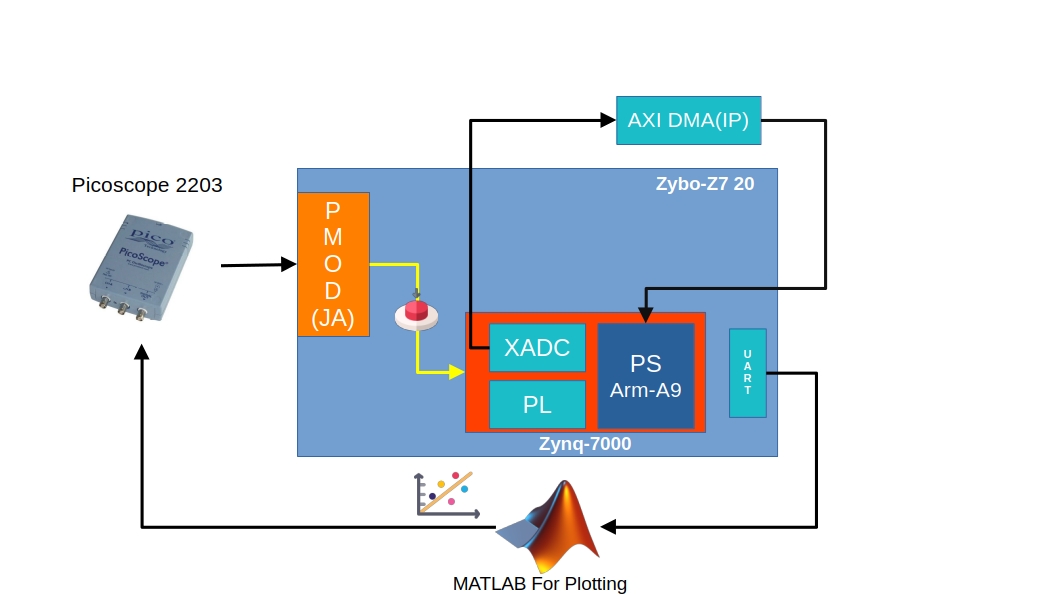
The differences between the two designs are visually represented in Figure 1 and Figure 2, highlighting the progression from the original implementation to the enhanced version.

Figure 1 depicts the initial design from the previous project, which relied on external tools like Putty for data capture and the PicoScope 7 SDK for signal generation. While functional, this setup involved multiple software dependencies and manual interventions, resulting in a more fragmented workflow.
Figure 2 illustrates the updated design in this project, showcasing the integration of MATLAB with PicoScope drivers for direct signal generation. Additionally, the serial communication for data transmission and reception has been streamlined within MATLAB itself, eliminating the need for external tools and simplifying the overall architecture.

These visual comparisons clearly demonstrate how the new design achieves a more cohesive and efficient workflow, reducing complexity while improving usability and performance.

Figure 1: Previous Design Flow

Figure 2: Revised Design Flow

Environment Setup

To replicate the implementation outlined in this project, you will need to install the following drivers in your MATLAB environment:

PicoScope Support Toolbox: This toolbox can be installed directly from MATLAB's Add-ons section. It provides essential support for integrating PicoScope functionality into MATLAB.
PicoScope 2000 Series MATLAB Generic Instrument Driver (according to your picoscope device): Also available in MATLAB's Add-ons section, this driver facilitates seamless communication with PicoScope devices.
Picoscope 7 SDK: This software development kit must be downloaded and installed from the official Pico Technology Store. It enables advanced configuration and control of PicoScope devices.

Ensure you have these components set up correctly to proceed with the implementation.

MATLAB GUI Creation

To get started with installing the required tools, follow these steps:

Open MATLAB and navigate to the menu bar.
Click on the Apps tab in the menu bar.
In the Apps menu, locate the option labeled Design App.
Click on Design App to proceed

Figure 3: Opening The Designer APP

This action will launch the App Designer interface in MATLAB.

Once the App Designer opens, select the option Blank App to start with a new, customizable application template.
From here, you can begin designing and configuring your app as per the requirements of this project.

Figure 4: App Designer Interface

In this step, you will add the necessary controls and functions to configure the Picoscope and receive data.

On the left-hand side of the App Designer, you’ll find the Component Library. In the Component Library, search for the following components:

Buttons: These will allow the user to trigger actions such as starting and stopping data acquisition.
Axes: These will display the signal data and plots.
Labels: These can be used to provide instructions or titles for your interface.

Drag and drop the following components onto your design canvas:

Two buttons: one for starting the signal acquisition and another for stopping or resetting the process.
Two axes: one for displaying the incoming signal data and the other for additional visualizations, such as frequency spectrum or processed data.
Two labels: one to describe the first button (e.g., "Start Acquisition") and another for the second button (e.g., "Stop Acquisition").

By arranging these components on the canvas, you’ll create the user interface needed to interact with the PicoScope hardware.

Figure 5: Adding Components

Figure 6 shows the usage of these components.

Figure 6: Component USAGE

In the App Designer, on the right-hand side, you'll find the Component Browser window. This is where you can customize the properties of each component you've added to your design.

Select the component you want to modify (e.g., a button, axis, or label) by clicking on it in the Design View.
In the Component Browser, you'll see various options for customization. You can adjust:
Size: Modify the width, height, and position of the component.
Text: Change the text displayed on buttons or labels (e.g., change "Start" to "Start Acquisition").
Font: Adjust the font type, size, and style for labels and buttons.
Other Properties: Customize other settings such as colors, borders, and alignment to fit your design.

These options allow you to personalize the appearance and layout of your interface to enhance usability and presentation.

Figure 7: App Designer Customization

After customizing the components, my final design now looks like the one shown in Figure 8. This updated interface includes all the necessary controls, axes, and labels, tailored to the requirements of the project. The design is visually optimized for ease of use and functionality.

Figure 8: APP Front-End

I have kept it as simple as possible. You can play around to make it more vibrant.

Adding Functionality To Our Front-End

Currently, our app is non-functional. Let's now add functionality to it.

Click on Button 1 in the Design View of the App Designer to select it.
In the Component Browser window on the right-hand side, scroll down and look for the Callbacks section.
Click on Callbacks to expand the options.
Find the callback function for Button 1 (it should be labeled something like Button1Pushed).
Click the Add Callback button to create a new callback function for the button.

This callback function will be triggered when the user presses Button 1. You can now write the code inside this function to configure the PicoScope, start signal acquisition, or perform any other necessary task based on your project requirements.

Figure 9: Adding Callbacks to button

Clicking on Add Callback will open the Code View in the App Designer, providing you with a space to enter your logic.

In this view, you’ll see the auto-generated code for the callback function tied to Button 1. You can now write your specific logic inside this function. For example, you could add commands to configure the PicoScope, start data acquisition, or trigger any other action related to the hardware or the app's functionality.

Additionally, App Designer automatically generates code for other components that you've added to your GUI (such as buttons, labels, and axes). You can edit this code as needed to implement your desired behavior, but the structure and functionality for basic component interactions are already set up for you.

In the provided space, enter the following code. The code includes in-line comments to explain its functionality:

%To clear are instruments conncetions previously present in MATLAB workspace
instrreset;
%array to store voltage data
app.VoltageData =[];
app.timeData=[];
%array to store sample count
app.sampleCount=0;
% Used to make the label1 you added in your design to display
% Replace StatusLabel with the name of your label1
app.StatusLabel.Text = 'Siganl generation started...';
app.sampleRate = 1000000;
%load picoscope configurations
PS2000Config;
%Conncet to picoscope device
app.ps2000DeviceObj = icdevice('picotech_ps2000_generic.mdd');
connect(app.ps2000DeviceObj);
% Signal Generator Configuration
sigGenGroupObj = get(app.ps2000DeviceObj, 'Signalgenerator');
sigGenGroupObj = sigGenGroupObj(1);
set(sigGenGroupObj, 'startFrequency', 50000); % Frequency in Hz
set(sigGenGroupObj, 'offsetVoltage', 400);%offset volatge
set(sigGenGroupObj, 'peakToPeakVoltage', 800); % Peak-to-peak voltage in mV
[status.sigGenSimple] = invoke(sigGenGroupObj, 'setSigGenBuiltInSimple', ...
ps2000Enuminfo.enPS2000WaveType.PS2000_SINE);
serialPort = '/dev/ttyUSB1';  % Replace with your correct port
app.serialObj = serial(serialPort, 'BaudRate', 115200, 'Terminator', 'LF', 'Timeout', 10);
fopen(app.serialObj);  % Open the serial port
% Real-time data collection loop
while (ishandle(app.UIAxes) && ~app.stopFlag) % Check if the figure is still open
data = fgetl(app.serialObj);
if ischar(data)
voltage = str2double(data);
if ~isnan(voltage)
app.sampleCount = app.sampleCount + 1;
app.VoltageData = [app.VoltageData, voltage];
app.timeData = [app.timeData, app.sampleCount];
% Clear the previous plot and plot the new data replace UIAxes with your axes1 % name
plot(app.UIAxes, app.timeData, app.VoltageData, '-o');
xlabel(app.UIAxes, 'Time (samples)');
ylabel(app.UIAxes, 'Voltage (V)');
title(app.UIAxes, 'Real-Time Voltage Data');
drawnow;
% Perform FFT on VoltageData
n = length(app.VoltageData); % Number of samples
if n >= 800 % Minimum number of samples to compute FFT (e.g., 1024)
% Compute the FFT
Y = fft(app.VoltageData);
f = (0:n-1)*(app.sampleRate/n);  % Frequency vector
% Plot the FFT (amplitude spectrum)
amplitude = abs(Y)/n; % Normalized amplitude
frequencyPlot = f(1:floor(n/2)); % Only the positive frequencies
amplitudePlot = amplitude(1:floor(n/2));
% Plot the FFT on a different axis (frequency domain plot)
% Replace UIAxes2 with the name of your second axes
plot(app.UIAxes2, frequencyPlot, amplitudePlot);
xlabel(app.UIAxes2, 'Frequency (Hz)');
ylabel(app.UIAxes2, 'Amplitude');
title(app.UIAxes2, 'Frequency Spectrum');
drawnow;
end
end
end
end
%replace label with name of your second label
app.Label.Text = 'Process has been stopped by user....';

In the above code, you may have noticed some variables are referenced as app.*. These variables are properties of the App class in MATLAB’s App Designer. The reason they are defined as app.* is that they are declared as properties in the Properties section of the GUI.

By declaring these variables as properties, they become accessible by other functions within the GUI. This allows different functions (such as callback functions, data processing, and UI updates) to share and modify these variables.

How to Define Properties:

Add Property in App Designer:

In the App Designer, go to the Code View.
In the Properties section of the Editor (usually located at the top of the code), click Add Property.

Space to Add Properties:

When you click Add Property, the editor will automatically provide a space in the Properties section where you can define these properties.

Once clicking to run my code the variables shown in Figure 10 need to be added.

So now everything is setup, and Voilà, you can run the app.

Hardware-In-Loop Simulation Demo

Thank you for your time and attention. If you have any queries or need further assistance, feel free to reach out to me. I will be happy to help you. 😊

Happy Learning and best of luck with your project! 🚀📚

Code

MATLAB GUI CODE

classdef HILGUI < matlab.apps.AppBase

    % Properties that correspond to app components
    properties (Access = public)
        UIFigure                 matlab.ui.Figure
        RevisedDesignFlowLabel   matlab.ui.control.Label
        Image2                   matlab.ui.control.Image
        PreviousDesignFlowLabel  matlab.ui.control.Label
        Image                    matlab.ui.control.Image
        Label                    matlab.ui.control.Label
        STOPReceptionButton      matlab.ui.control.Button
        StatusLabel              matlab.ui.control.Label
        StartReceptionButton     matlab.ui.control.Button
        UIAxes2                  matlab.ui.control.UIAxes
        UIAxes                   matlab.ui.control.UIAxes
    end

    
    properties (Access = private)
        VoltageData
        timeData
        sampleCount% Description
        ps2000DeviceObj
        serialObj% Description
        stopFlag = false; % Description
        sampleRate; % Description
    end
    

    % Callbacks that handle component events
    methods (Access = private)

        % Button pushed function: StartReceptionButton
        function StartReceptionButtonPushed(app, event)
                instrreset;
                app.VoltageData =[];
                app.timeData=[];
                app.sampleCount=0;
                app.StatusLabel.Text = 'Siganl generation started...';
                app.sampleRate = 1000000;
                %load picoscope configurations
                PS2000Config;

                %Conncet to picoscope device
                app.ps2000DeviceObj = icdevice('picotech_ps2000_generic.mdd');
                connect(app.ps2000DeviceObj);
                % Signal Generator Configuration
                sigGenGroupObj = get(app.ps2000DeviceObj, 'Signalgenerator');
                sigGenGroupObj = sigGenGroupObj(1);
                set(sigGenGroupObj, 'startFrequency', 50000); % Frequency in Hz
                set(sigGenGroupObj, 'offsetVoltage', 400);
                set(sigGenGroupObj, 'peakToPeakVoltage', 800); % Peak-to-peak voltage in mV
                [status.sigGenSimple] = invoke(sigGenGroupObj, 'setSigGenBuiltInSimple', ...
                ps2000Enuminfo.enPS2000WaveType.PS2000_SINE);

                serialPort = '/dev/ttyUSB1';  % Replace with your correct port
                app.serialObj = serial(serialPort, 'BaudRate', 115200, 'Terminator', 'LF', 'Timeout', 10);
                fopen(app.serialObj);  % Open the serial port

                % Real-time data collection loop
                
                    
                while (ishandle(app.UIAxes) && ~app.stopFlag) % Check if the figure is still open
                data = fgetl(app.serialObj);
        
                if ischar(data)
                voltage = str2double(data);
            
                if ~isnan(voltage)
                app.sampleCount = app.sampleCount + 1;
                app.VoltageData = [app.VoltageData, voltage];
                app.timeData = [app.timeData, app.sampleCount];
                
                % Clear the previous plot and plot the new data
                plot(app.UIAxes, app.timeData, app.VoltageData, '-o');
                xlabel(app.UIAxes, 'Time (samples)');
                ylabel(app.UIAxes, 'Voltage (V)');
                title(app.UIAxes, 'Real-Time Voltage Data');
                drawnow;
                % Perform FFT on VoltageData
                n = length(app.VoltageData); % Number of samples
                if n >= 800 % Minimum number of samples to compute FFT (e.g., 1024)
                    % Compute the FFT
                    Y = fft(app.VoltageData);
                    f = (0:n-1)*(app.sampleRate/n);  % Frequency vector

                    % Plot the FFT (amplitude spectrum)
                    amplitude = abs(Y)/n; % Normalized amplitude
                    frequencyPlot = f(1:floor(n/2)); % Only the positive frequencies
                    amplitudePlot = amplitude(1:floor(n/2));

                    % Plot the FFT on a different axis (frequency domain plot)
                    plot(app.UIAxes2, frequencyPlot, amplitudePlot);
                    xlabel(app.UIAxes2, 'Frequency (Hz)');
                    ylabel(app.UIAxes2, 'Amplitude');
                    title(app.UIAxes2, 'Frequency Spectrum');
                    drawnow;
                end
                end
                end
                end

                app.Label.Text = 'Process has been stopped by user....';
        end

        % Button pushed function: STOPReceptionButton
        function STOPReceptionButtonPushed(app, event)
            app.stopFlag = true;
            instrreset;
        end
    end

    % Component initialization
    methods (Access = private)

        % Create UIFigure and components
        function createComponents(app)

            % Get the file path for locating images
            pathToMLAPP = fileparts(mfilename('fullpath'));

            % Create UIFigure and hide until all components are created
            app.UIFigure = uifigure('Visible', 'off');
            app.UIFigure.Position = [100 100 1663 823];
            app.UIFigure.Name = 'MATLAB App';

            % Create UIAxes
            app.UIAxes = uiaxes(app.UIFigure);
            title(app.UIAxes, 'Voltage Time Plot')
            xlabel(app.UIAxes, 'Sample Count')
            ylabel(app.UIAxes, 'Voltage Values')
            zlabel(app.UIAxes, 'Z')
            app.UIAxes.LineWidth = 0.7;
            app.UIAxes.Box = 'on';
            app.UIAxes.Position = [57 333 428 267];

            % Create UIAxes2
            app.UIAxes2 = uiaxes(app.UIFigure);
            title(app.UIAxes2, 'Title')
            xlabel(app.UIAxes2, 'X')
            ylabel(app.UIAxes2, 'Y')
            zlabel(app.UIAxes2, 'Z')
            app.UIAxes2.Position = [564 324 409 276];

            % Create StartReceptionButton
            app.StartReceptionButton = uibutton(app.UIFigure, 'push');
            app.StartReceptionButton.ButtonPushedFcn = createCallbackFcn(app, @StartReceptionButtonPushed, true);
            app.StartReceptionButton.Icon = fullfile(pathToMLAPP, 'button_blank_blue_14984.png');
            app.StartReceptionButton.BackgroundColor = [1 1 1];
            app.StartReceptionButton.FontSize = 18;
            app.StartReceptionButton.Position = [430 689 226 54];
            app.StartReceptionButton.Text = 'Start Reception';

            % Create StatusLabel
            app.StatusLabel = uilabel(app.UIFigure);
            app.StatusLabel.HorizontalAlignment = 'center';
            app.StatusLabel.FontSize = 18;
            app.StatusLabel.FontColor = [0 1 0];
            app.StatusLabel.Position = [432 617 221 39];
            app.StatusLabel.Text = '';

            % Create STOPReceptionButton
            app.STOPReceptionButton = uibutton(app.UIFigure, 'push');
            app.STOPReceptionButton.ButtonPushedFcn = createCallbackFcn(app, @STOPReceptionButtonPushed, true);
            app.STOPReceptionButton.BackgroundColor = [1 0 0];
            app.STOPReceptionButton.FontSize = 18;
            app.STOPReceptionButton.FontColor = [1 1 1];
            app.STOPReceptionButton.Position = [452 213 182 52];
            app.STOPReceptionButton.Text = 'STOP Reception';

            % Create Label
            app.Label = uilabel(app.UIFigure);
            app.Label.FontSize = 18;
            app.Label.Position = [340 150 406 29];
            app.Label.Text = '';

            % Create Image
            app.Image = uiimage(app.UIFigure);
            app.Image.Position = [760 445 1068 298];
            app.Image.ImageSource = fullfile(pathToMLAPP, 'XADC.jpg');

            % Create PreviousDesignFlowLabel
            app.PreviousDesignFlowLabel = uilabel(app.UIFigure);
            app.PreviousDesignFlowLabel.HorizontalAlignment = 'center';
            app.PreviousDesignFlowLabel.FontSize = 24;
            app.PreviousDesignFlowLabel.FontWeight = 'bold';
            app.PreviousDesignFlowLabel.Position = [1158 757 271 31];
            app.PreviousDesignFlowLabel.Text = 'Previous Design Flow';

            % Create Image2
            app.Image2 = uiimage(app.UIFigure);
            app.Image2.Position = [792 35 1004 299];
            app.Image2.ImageSource = fullfile(pathToMLAPP, 'XADCrev.jpg');

            % Create RevisedDesignFlowLabel
            app.RevisedDesignFlowLabel = uilabel(app.UIFigure);
            app.RevisedDesignFlowLabel.HorizontalAlignment = 'center';
            app.RevisedDesignFlowLabel.FontSize = 24;
            app.RevisedDesignFlowLabel.FontWeight = 'bold';
            app.RevisedDesignFlowLabel.Position = [1175 344 273 54];
            app.RevisedDesignFlowLabel.Text = 'Revised Design Flow';

            % Show the figure after all components are created
            app.UIFigure.Visible = 'on';
        end
    end

    % App creation and deletion
    methods (Access = public)

        % Construct app
        function app = HILGUI

            % Create UIFigure and components
            createComponents(app)

            % Register the app with App Designer
            registerApp(app, app.UIFigure)

            if nargout == 0
                clear app
            end
        end

        % Code that executes before app deletion
        function delete(app)

            % Delete UIFigure when app is deleted
            delete(app.UIFigure)
        end
    end
end

Credits

Saqib Awan

3 projects • 5 followers

Hardware Engineer and Embedded Systems Enthusiast | Passionate about SoCs, RFSoCs, and Cutting-Edge Hardware Design

Contact

Comments

Please log in or sign up to comment.

Hardware-in-the-Loop Simulation with MATLAB and Zyob-Z7

Things used in this project

Hardware components

Software apps and online services

Story

Environment Setup

MATLAB GUI Creation

Adding Functionality To Our Front-End

How to Define Properties:

Schematics

Final Block Design

Code

MATLAB GUI CODE

Credits

Saqib Awan

Comments

Embed the widget on your own site

Hardware-in-the-Loop Simulation with MATLAB and Zyob-Z7

Hardware-in-the-Loop Simulation with MATLAB and Zyob-Z7

Things used in this project

Hardware components

Software apps and online services

Story

Environment Setup

MATLAB GUI Creation

Adding Functionality To Our Front-End

How to Define Properties:

Schematics

Final Block Design

Code

MATLAB GUI CODE

Credits

Saqib Awan

Comments

Related channels and tags